Example:

Description:

                There are *MANY* missing indicators. I have not had the strength
                to tackle this section yet.
                
                Missing From MetaStock
                - Absolute Open to close change percent



                Missing from StockFetcher
                Accumulation Swing Index


            

Example:

Description:

                A measure of a stock's closing price relative to the open.
                The value is the difference between the close and open, 
                represented as a percent of the opening price.

                While you can refer to all of them using the longer syntax 
                "Absolute Open to Close Change Percent", the examples below show 
                the "abbreviated" versions.

                show stocks where the opcl is above 0

                show stocks where the opcl% is below -2.5%

                show stocks where the aopcl is above 2.0

                show stocks where the aopcl% is above 5.0%

                In summary:

                • opcl = Open to Close Change 
                • opcl% = Open to Close Change Percent
                • aopcl = Absolute Open to Close Change
                • aopcl% = Absolute Open to Close Change Percent
                
                Formula:
                    opcl = close - open
                    
                    aopcl = abs(close - open)
                    
                    opcl% = 100 * ((CLOSE - OPEN)/CLOSE)
                    
                    aopcl% = abs(100 * ((CLOSE - OPEN)/CLOSE))
            

Example:

Description:

Learn More

                The Absolute Price Oscillator (APO) is the exact same measure as
                the Percent Price Oscillator (PPO) except the values are not
                converted to percentages. The APO is computed by taking the
                difference between two specified moving averages.
            

Example:

Description:

Learn More

                The Absolute Volume Oscillator (AVO) computes the difference
                between two average volume measures. Unlike the Percent Volume
                Oscillator(PVO) the AVO does not convert the difference to a
                percent or normalize the results.

                Formula:
            

Example:

Description:

                Developed by Price Headley, the Acceleration bands are based on
                the average trading range for each day. The values are plotted
                equidistant from an n-day simple moving average which serves as
                the center or middle band. The author indicates that successive
                days exceeding one of the bands tends to indicate an entry
                point.

                Because the bands use the daily trading range (high-low) they
                will also expand and contract based on the volatility of the
                price.
            

Amazon: Big Trends In Trading By Price Headly

Example:

Description:

Learn More

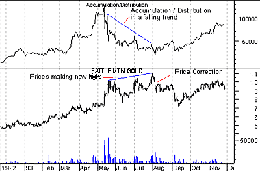
                There are many indicators available to measure volume and the flow
                of money for a particular stock, index or security. One of the most
                popular volume indicators over the years has been the
                Accumulation/Distribution Line. The basic premise behind volume
                indicators, including the Accumulation/Distribution Line, is that
                volume precedes price. Volume reflects the amount of shares traded
                in a particular stock and is a direct reflection of the money
                flowing into and out of a stock. Many times before a stock advances,
                there will be period of increased volume just prior to the move.
                Most volume or money flow indicators are designed to identify early
                increases in positive or negative volume flow to gain an edge before
                the price moves. (Note: the terms "money flow" and "volume flow" are
                essentially interchangeable.)

                Methodology

                The Accumulation/Distribution Line was developed by Marc Chaikin to
                assess the cumulative flow of money into and out of a security. In
                order to fully appreciate the methodology behind the
                Accumulation/Distribution Line, it may be helpful to examine one of the
                earliest volume indicators and see how it compares.

                Example
            

                In 1963, Joe Granville developed On Balance Volume (OBV), which was
                one of the earliest and most popular indicators to measure positive
                and negative volume flow. OBV is a relatively simple indicator that
                adds the corresponding period's volume when the close is up and
                subtracts it when the close is down. A cumulative total of the
                positive and negative volume flow (additions and subtractions) forms
                the OBV line. This line can then be compared with the price chart
                of the underlying security to look for divergences or confirmation.

                In developing the Accumulation/Distribution Line, Chaikin took a
                different approach. OBV uses the change in closing price from one
                period to the next to value the volume as positive or negative.
                Even if a stock opened on the low and closed on the high, the period's
                OBV value would be negative as long as the close was lower than the
                previous period's close. Chaikin choose to ignore the change from
                one period to the next and instead focused on the price action for
                a given period (day, week, month). He derived a formula to calculate
                a value based on the location of the close, relative to the range for
                the period. We will call this value the "Close Location Value" or CLV.
                The CLV ranges from plus one to minus one with the center point at zero.
                There are basically five combinations:


                1. If the stock closes on the high, the absolute top of the range,
                then the value would be plus one.

                2. If the stock closes above the midpoint of the high-low range, but
                below the high, then the value would be between zero and one.

                3. If the stock closes exactly halfway between the high and the low,
                then the value would be zero.

                4. If the stock closes below the midpoint of the high-low range, but
                above the low, then the value would be negative.

                5. If the stock closes on the low, the absolute bottom of the range,
                then the value would be minus one.

                The CLV is then multiplied by the corresponding period's volume and
                the cumulative total forms the Accumulation/Distribution Line.

                Bullish Signals

                A bullish signal is given when the Accumulation/Distribution Line
                forms a positive divergence. Be wary of weak positive divergences
                that fail to make higher reaction highs or those that are relatively
                young. The main issue is to identify the general trend of the
                Accumulation/Distribution Line. A two-week positive divergence may
                be a bit suspect. However, a multi-month positive divergence
                deserves serious attention.

                Bearish Signals

                The same principles that apply to positive divergences apply to
                negative divergences. The key issue is to identify the main trend
                in the Accumulation/Distribution Line and compare it to the underlying
                security. Young negative divergences, or those that are relatively
                flat, should be looked upon with a healthy dose of skepticism.

                Formula:

                A portion of each day's volume is added or subtracted from a cumulative
                total. The nearer the closing price is to the high for the day, the
                more volume added to the cumulative total. The nearer the closing
                price is to the low for the day, the more volume subtracted from the
                cumulative total. If the close is exactly between the high and low
                prices, nothing is added to the cumulative total.
            

Example:

Description:

                By default, StockFetcher returns basic price and volume
                information for each of the stocks returned in a screen.

                This information includes:

                •    most recent closing price.
                •    percent change from previous close.
                •    the number of shares traded during the
                most recent day.

                The results columns can easily be augmented using the add column
                phrase. With add column nearly any measure or indicator may be
                added to the filter results. As an example, the ten day average
                volume is added as a column to a basic stock screen:

                Price is between 10 and 50
                and Add column average volume(10)

                Now the results present the ten day average volume along with
                the standard information.

                In addition to providing new information with the filter
                results, each new measure can be sorted in either ascending or
                descending order by clicking on the appropriate column header.
                Sorting these additional columns is useful with measures whose
                high or low values can provide additional approach confirmation.
                For example, take an approach where the close-to-open gap in
                price is displayed.

                Show stocks where the price is between 10 and 15
                and Add column close to open gap

                Clicking on the column heading for the "close to open gap"
                immediately presents the results where the most recent open
                price gapped significantly from the closing price the day
                before.

                Column Aliases

                Enclosing text inside the {} symbols provides an optional
                extension to the "add column" phrase. These braces are used to
                rename resulting column headers to something more concise or
                meaningful. Taking the average volume example above, suppose the
                column is renamed to "av10" to clean up the results.

                Price is between 10 and 50
                and Add column average volume(10) {av10}

                The contents inside the {...} will be used as the new column
                header. This extension definitely proves useful when many
                measures are added to the results, or when the actual measures
                added to the results are complex and produce difficult to read
                headers. In the example below, a 52-week high of the MA(50) is
                added to the results.

                Price is between 10 and 50
                and Add column average volume(10) {av10}
                and Add column MA(50) 52 week high {ma50hi}
            

Example:

Description:

                The A/D Ratio is similar to the Advancing-Declining Issues in that it
                displays market breadth. But, where the Advancing-Declining Issues
                subtracts the advancing/declining values, the A/D Ratio divides the
                values. The advantage of the Ratio is that it remains constant
                regardless of the number of issues that are traded on the
                New York Stock Exchange (which has steadily increased).

                A moving average of the A/D Ratio is often used as an
                overbought/oversold indicator. The higher the value, the more
                "excessive" the rally and the more likely a correction. Likewise, low
                readings imply an oversold market and suggest a technical rally.

                Keep in mind, however, that markets that appear to be extremely
                overbought or oversold may stay that way for some time. When
                investing using overbought and oversold indicators, it is wise to
                wait for the prices to confirm your belief that a change is due before
                placing your trades.

                Day-to-day fluctuations of the Advance/Decline Ratio are often
                eliminated by smoothing the ratio with a moving average.

                Formula:
            

               The A/D Ratio is calculated by dividing the number of stocks that
                advanced in price for the day by the number of stocks that declined.

                This indicator was revisited in December 2004 issue of Technical Analysis of Stocks & Commodities
                magazine pg 68 by Tom McClellan.
            

Example:

Description:

More Watch List Information

                By default, StockFetcher will scan all stocks when performing a
                screen. Sometimes, it isn't necessary to see all matches. As an
                example, when developing an exit strategy, it is helpful to look
                at specific stocks that have already met an entry requirement.
                On StockFetcher, this is accomplished by applying a filter
                specifically to a list of stocks called the watch list.

                Simply adding the phrase apply to watch list tells StockFetcher
                to scan stocks in the watch list. For example the following phrase

                MA(50) crossed above MA(200) And apply to watch list

                provides the crossover as an exit condition, but only for the
                stocks that are currently in the watch list.

            

Example:

Description:

Learn More

Learn More

                The Arms Index is an indicator that uses advancing and declining
                stocks and their volume to measure intra-day market supply
                demanddemand and can be applied over short or longer time periods.
                The Arms Index is named after its creator Richard W. Arms and is
                also know as the "TRIN" index   The formula is simple and can be
                applied to any index for which the data is available.  It is simply
                (Advancing issues/Declining issues) / (Advancing volume/ Declining
                volume).

                If more volume goes into advancing issues than declining issues the
                Arms Index falls below 1.0.  If more volume goes into declining
                stocks than advancing stocks the Arms Index rises above 1.0.

                Notes on the Arms Index

                • For the Arms Index, readings over 1.00 are bearish, but
                extreme readings may indicate that a market reversal is near.
                In general, any time the index gets over 2.5, a rally could occur
                near term.

                The caution is to never rely on one indicator and to have a strong
                fundamental understanding of why the current market trend is in
                place and what reasons if any might emerge that could change the
                current perceptions on fundamental valuations.  From a technical
                standpoint it is best to wait for price confirmation before trading
                or a strengthened argument by looking at other indicators and market
                data.

                • The Arms Index was created by relating the volume of
                advancing issues to the volume of declining issues. Generally a
                healthy volume accompanying a rise in prices is the forerunner of a
                better market than low volume.

                • Using moving averages of the index is one way to smooth the
                Arms Index.  Some traders look for moving average crossovers or zero
                line crossovers in developing trading uses for the Arms Index.

                • Usually numbers between zero and one are Bullish, while
                numbers above 1 are bearish.

                • Interpretation : 0-1  -- Bullish               >1  -- Bearish

                • Diverging plots of price/volume against the Arms Index can
                be an indication of a loss in Momentum.


                Formula:

                The Arms Index is calculated by first dividing the number of stocks
                that advanced in price by the number of stocks that declined in price
                to determine the Advance/Decline Ratio. Next, the volume of advancing
                stocks is divided by the volume of declining stocks to determine the
                Upside/Downside Ratio. Finally, the Advance/Decline Ratio is divided
                by the Upside/Downside Ratio.
            

Amazon: The Arms Index By Richard W., Jr. Arms

Example:

Description:

Learn More

                Used to detect potential trends in stocks, the aroon measures
                (developed by T. Chande) compute the amount of time since a closing
                value reached a new high or new low. Given a specified period,
                the aroon Up will search for the highest closing value during that
                period and return the distance from the most recent day for when
                that high happened. The aroon Down works in the same way except
                looking for the lowest closing vlaue. Finally, the aroon Oscillator
                simply takes the difference between the two values. Valid ranges for
                the aroon Up and aroon Down are 0-100 and for the aroon Oscillator
                the valid range is -100 to 100.

                Aroon means "Dawn's Early Light" in Sanskrit. September 1995 issue of
                Technical Analysis of Stocks & Commodities magazine.

            

Example:

Description:

Learn More

                Developed by J. Welles Wilder and introduced in his book, New Concepts in Technical Trading Systems (1978).

                Using the relationships between the high and low of a day
                compared with the previous close, the Average True Range is a
                measure of volatility developed by Welles Wilder. Typically
                used to identify oversold and overbought conditions, a low
                average true range indicates a stock which lacks volatility,
                while high average true range indicates potentials sell-offs
                of a stock.

                Formula:
            

Amazon: New Concepts in Technical Trading Systems By J. Welles Wilder

Example:

Description:

                A simple average of the shares traded (volume) of a stock over
                the given number of days.

            

Example:

Description:

                Editors Note:

                Although this is not an idicator it is a fairly singificant
                usage pattern that almost makes SF backtesting usable.

                Thank you Cegis for the great insight that you continually provide.
                --------------------------------------------------------------------

                Original Post

                cegis 	9/17/2004 5:23:18 PM

                This is a discussion of a technique that I (cegis) developed
                a few months back, and has seemed to be useful regularly in
                other threads ever since. So, I decided to document it, in
                the hope it will be of use to others.

                This technique allows you to calculate returns for a filter,
                for any time period, and (almost) any assumed trading "program".

                What StockFetcher offers as basic site functionality is a
                column labeled "Performance" when showing results from a
                filter that has the "offset" phrase. The performance shown
                (I think - correct me if I'm wrong) is based on the closing
                price of the stock on the day that the stock matched the
                filter (the offset date) and yesterday's close. This means
                that the period covered by the column changes with the offset.
                You can also get the 1 day, 2 day, 3 day, 4 day, one week,
                two week, etc. performance for the filter's results by
                clicking on the Performance column header, and "browsing
                through the dates" (assuming there have been that many
                trading days in the offset period). This is good, but limiting.

                The scenarios that SF's Performance functionality does not
                take into account are things like "performance for a 10 day
                period, regardless of the start date", "worst case performance"
                using the day-after-match's high and end-of-period low as
                entry/exit points, or "trading program rules" such as max
                loss of 2%. This technique allows such analysis.

                The "trick" to this technique is to use the "days ago" phrase
                instead of the "offset" phrase. This allows you to "see what
                happened" AFTER the stocks matched your filter. As an example,
                if you use "offset 10 days", SF will not allow you to retrieve
                ("see") values from what would be "offset 9 days". However,
                if you use "10 days ago", you can always analyze what happened
                "9 days ago".

                Let's look at a simple example. We'll assume our starting filter is:

                rsi(2) is less than 1
                and price is between 1 and 10
                and average volume(25) is greater than 100000


                If we run this filter on Sat. 9/25/04 (which will be our assumed
                run date for all of the following discussion), we'll see the
                results for 9/24 market close. Now, let's assume we want to
                see how this filter performed based on picks from 10 days ago.
                If we use

                rsi(2) is less than 1
                and price is between 1 and 10
                and average volume(25) is greater than 100000
                offset 10 days


                we'll get selections for 9/10, and we'll get the Performance
                column talked about above (9/10 to 9/24, close to close), as
                standard SF functionality. However, if we wanted to see what
                a "worst case" scenario would have been, we would not be able
                to access the data for 9/11's high or 9/24's low to make this
                determination. However, if we instead used

                rsi(2) 10 days ago is less than 1
                and price 10 days ago is between 1 and 10
                and average volume(25) 10 days ago is greater than 100000


                we'll still get the results of our original filter as of 9/10,
                but now we can calculate our worst case scenario:

                set{myrtn,low - high 9 days ago}
                set{myrtnp,myrtn / high 9 days ago}
                set{wcrtnpct,myrtnp * 100}

                rsi(2) 10 days ago is less than 1
                and price 10 days ago is between 1 and 10
                and average volume(25) 10 days ago is greater than 100000

                add column high 9 days ago {entry}
                add column low {exit}
                add column myrtn {profit}
                add column wcrtnpct {profit percent}


                Since all of our conditions have "10 days ago", the first
                set{} command is "looking into the future" to get the following
                day's high (high 9 days ago), and the 10th day's low
                (low [0 days ago]), to calculate the return ($). The other two
                set{}s just convert the first set{} into a percentage. (I'm
                using my entry as the basis for the percentage...) The add
                columns will show us our result.

                Note that the return calculated will ALWAYS be a ten-day
                return. We can continue to backtest this filter by adding
                an "offset" too!

                set{myrtn,low - high 9 days ago}
                set{myrtnp,myrtn / high 9 days ago}
                set{wcrtnpct,myrtnp * 100}

                rsi(2) 10 days ago is less than 1
                and price 10 days ago is between 1 and 10
                and average volume(25) 10 days ago is greater than 100000

                add column high 9 days ago {entry}
                add column low {exit}
                add column myrtn {profit}
                add column wcrtnpct {profit percent}

                offset 1


                With the offset 1, we'll actually match stocks for 9/9, and
                show what the 10 day return is through 9/23. You can then
                alter the offset to continue backtesting other dates. In
                other words, you do NOT have to keep changing the "days ago"
                in order to backtest prior dates. Just remember that SF will
                report "results as of 9/24" (or whatever your offset would
                suggest) at the top of the results list, and you have to
                remeber that you used "days ago" to shift the data back an
                additional 10 days.

                Also note that you can calcualte multiple returns for the
                period covered by the "days ago" offset:

                set{myrtn10,low - high 9 days ago}
                set{myrtn10p,myrtn10 / high 9 days ago}
                set{wc10rtnpct,myrtn10p * 100}

                set{myrtn5,low 5 days ago - high 9 days ago}
                set{myrtn5p,myrtn5 / high 9 days ago}
                set{wc5rtnpct,myrtn5p * 100}

                rsi(2) 10 days ago is less than 1
                and price 10 days ago is between 1 and 10
                and average volume(25) 10 days ago is greater than 100000

                add column wc5rtnpct
                add column wc10rtnpct


                Here, we added a claculation of the 5 day worst case scenario,
                in addition to the 10 day return.

                This can be taken one step further (this is where this gets
                REALLY interesting!) by using "logical variables" to actually
                implement a "trading program". (Logical variables are discussed
                in several other threads, so I'm not gonna go into them here...)
                Let's say that you want a 2% trailing stop, and you'll hold
                for a max of 3 days. (I'll discuss this day limit later.)
                We'll assume we enter at the opening price, and exit at our
                stop or 3 day close. We'll also assume we only adjust our
                stop once a day based on the open. This filter will show you
                how well you would do:

                set{limit1,open 2 days ago * 0.98}
                set{in1,count(low 2 days ago is greater than limit1,1)}
                set{stopped1,1 - in1}
                set{out1,stopped1 * limit1}

                set{limit2, open 1 day ago * 0.98}
                set{in2,count(low 1 day ago is greater than limit2,1) * in1}
                set{stopped2a,1 - in2}
                set{stopped2,stopped2a * in1}
                set{out2,stopped2 * limit2}

                set{limit3, open * 0.98}
                set{in3,count(low is greater than limit3,1) * in2}
                set{stopped3a,1 - in3}
                set{stopped3,stopped3a * in2}
                set{out3,stopped3 * limit3}

                set{out3c,close * in3}

                set{outa,out1 + out2}
                set{outb,outa + out3}
                set{out,outb + out3c}

                add column open 2 days ago {in}
                add column out1
                add column out2
                add column out3
                add column out3c

                rsi(2) 3 days ago is less than 1
                and price 3 days ago is between 1 and 10
                and average volume(25) 3 days ago is greater than 100000


                So here, out1, out2, out3, and out3c will show you your exit
                price if you exit on the first, second, or third days, or at
                the close of the third day (respectively). They will be ZERO
                if you did not exit on that day. Thus, you can see when you
                would have exited, as well as how well you would have done.

                There are two things I would have liked to do in the prior
                filter, but SF limits how many times you can "nest" set{}
                statements (that is, base one set{} on the results of another).
                I would have liked to change the calculation of limit2 and
                limit3 so that it only goes up in value (a trailing stop),
                as well as calcaulte the $ and percentage return based on my
                exit price. I would have also liked to check for "green hold"
                (high 2 days ago > close 3 day ago) before considering myself
                "in". However, this filter sits right at the edge of the SF
                nesting limit, so I was unable to do that. That's also why I
                chose a three day maximum hold period.

                One way to get around this, somewhat, is to show results for
                every day (instead of figuring out if you would have been
                stopped), like this:

                set{limit, open 9 days ago * 0.98}

                set{profit1, high 9 days ago * 0.98}
                set{profit2, high 8 days ago * 0.98}
                set{profit3, high 7 days ago * 0.98}
                set{profit4, high 6 days ago * 0.98}
                set{profit5, high 5 days ago * 0.98}
                set{profit6, high 4 days ago * 0.98}
                set{profit7, high 3 days ago * 0.98}
                set{profit8, high 2 days ago * 0.98}
                set{profit9, high 1 days ago * 0.98}

                add column open 9 days ago {in}
                add column limit
                add column low 9 days ago {low1}
                add column profit1
                add column low 8 days ago {low2}
                add column profit2
                add column low 7 days ago {low3}
                add column profit3
                add column low 6 days ago {low4}
                add column profit4
                add column low 5 days ago {low5}
                add column profit5
                add column low 4 days ago {low6}
                add column profit6
                add column low 3 days ago {low7}
                add column profit7
                add column low 2 days ago {low8}
                add column profit8
                add column low 1 days ago {low9}
                add column profit9

                rsi(2) 10 days ago is less than 1
                and price 10 days ago is between 1 and 10
                and average volume(25) 10 days ago is greater than 100000


                Now, you can read across the columns, and if you assume you
                use 2% below the high as the following day's stop, all you
                have to do is read across the columns to see where a "low"
                value is less than the prior column (profit or limit) to see
                where you would have been stopped out.

                This isn't perfect, but it can get you some useful information!

                Things to Consider
                ==================
                • The number of days you want to use in the "days ago" phrase
                is the maximum holding period (or days worth of data you need)
                to calculate your returns. You do not want to use a larger number.

                • If your filter compares to prior days (ie, something like
                "open is greater than close 1 day ago"), you want to ADD
                the number of days in this calculationally-based days ago
                to the condition's days ago (in this case, making it something
                like "open 10 days ago is greater than close 11 days ago").

                • Note that the days ago prevents you from running the backtest
                as of a date "closer" to today than the number of days ago
                used. I do not consider this a major limiting factor.

                • SF will report "Filter results for [day of week] [date]".
                This will be based on the offset, not your days ago, value.
                You just need to remember that you have programmed an
                additional offset into the filter for backtesting purposes.

                • Whenever I use this technique, I first copy the filter that
                I want to backtest, then modify it to do the calculations
                and use the days ago that I need. You don't really want to
                use days ago (in the manner described here) in a filter
                you're gonna actually select stocks from...

                • Depending on your trading conditions and return calculations,
                you may be able to use the count() and sum() functions,
                and/or the "[n] days high" / "[n] days low", to look at
                longer time frames than the three days as in the example.

                • If you are backtesting a weekly filter, use "weeks ago"
                instead of "days ago". Also, funky things will happen
                if your filter mixes weekly and daily indicators.
                (Basically, the "days ago" and "offset" are not quite
                equivalent due to the way SF handles weekly values...)

                • Remember that you can download the results into a spreadsheet,
                and then use that to extend the backtest based on any
                logic you couldn't get into the filter.

                Hope this helps,

                C
            

Example:

Description:

Learn More

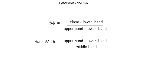
                The Bollinger %B analyzes the current price of a stock with
                respect to the width of it's Bollinger Bands. By subtracting the
                price from the lower band and dividing by the actual band width,
                the Bollinger %B provides an oscillator that can detect the
                stock's position within the bands.

                Formula:
            

Amazon: Bollinger on Bollinger Bands by John A. Bollinger

Example:

Description:

Learn More

Learn More

                Bollinger Bands are similar to moving average envelopes. The
                difference between Bollinger Bands and envelopes is envelopes are
                plotted at a fixed percentage above and below a moving average,
                whereas Bollinger Bands are plotted at standard deviation levels
                above and below a moving average. Since standard deviation is a
                measure of volatility, the bands are self-adjusting: widening during
                volatile markets and contracting during calmer periods.

                Bollinger Bands were created by John Bollinger.

                Interpretation

                Bollinger Bands are usually displayed on top of security prices, but
                they can be displayed on an indicator. These comments refer to bands
                displayed on prices.

                As with moving average envelopes, the basic interpretation of
                Bollinger Bands is that prices tend to stay within the upper- and
                lower-band. The distinctive characteristic of Bollinger Bands is
                that the spacing between the bands varies based on the volatility
                of the prices. During periods of extreme price changes (i.e., high
                volatility), the bands widen to become more forgiving. During
                periods of stagnant pricing (i.e., low volatility), the bands
                narrow to contain prices.

                Mr. Bollinger notes the following characteristics of Bollinger Bands.

                • Sharp price changes tend to occur after the bands tighten,
                as volatility lessens.

                • When prices move outside the bands, a continuation of the
                current trend is implied.

                • Bottoms and tops made outside the bands followed by bottoms
                and tops made inside the bands call for reversals in the trend.

                • A move that originates at one band tends to go all the way
                to the other band. This observation is useful when projecting
                price targets.

                Formula:
            

Amazon: Bollinger on Bollinger Bands by John A. Bollinger

Example:

Description:

Learn More

Learn More

                The Bollinger Width Oscillator is a simple extension of the
                Bollinger Bands using the closing price. Essentially the
                Bollinger Width Oscillator computes the position of the
                closing price relative to the width of the Bollinger Bands.

                This oscillator ranges from -100 to 100. Where a value above
                100 indicates the closing price is above the upper band and a
                value of -100 would indicate the price is below the lower band.
                Similarly, a value at 0 indicates the price is centered on the
                median Bollinger line (or moving average.)
            

Amazon: Bollinger on Bollinger Bands by John A. Bollinger

Example:

Description:

Learn More

Learn More

                The Bollinger Width returns the width of the upper and lower
                bollinger band divided by the n-day average price. In
                other words, a Bollinger width near 0 indicates the upper and
                lower bollinger bands are very close together while a value
                near 1 indicates wide bands.
            

Amazon: Bollinger on Bollinger Bands by John A. Bollinger

Example:

Description:

                Editors Note:

                Although this is not an idicator it does provide functionality
                this is not directly supported.
                --------------------------------------------------------------------

                Original Post

                TheRumpledOne 	8/24/2003 1:25:46 PM

                I have implemented OR, NOT and AND using SF set and count
                functions. Now we have a complete logic system within SF. THERE
                IS NOTHING YOU CAN'T DO NOW!

                This should revolutionize SF Filter writing.

                /* OR Implementation */
                /* by definition OR is TRUE IF A is TRUE, B is TRUE, or A AND B is TRUE*/
                /* THEREFORE by counting and adding, if the sum is greater */
                /* than 0 the OR condition is TRUE. */
                /* Copyright 2003 by Avery T. Horton, Jr. */
                /* Permission to use OR Implementation withing StockFetcher Granted */
                /* Permission to publish or post on any other forum DENIED */
                /* ----------------------------------------------------------------*/
                set{A, count(close above 100, 1)}
                set{B, count(volume above 50,000,000, 1)}
                set{OR1, A + B} show stocks where OR1 above 0


                /* NOT Implementation */
                /* by definition NOT A is TRUE IF A is FALSE*/
                /* THEREFORE by counting and adding, if the sum is equal to 0 */
                /* the NOT condition is TRUE. */
                /* Copyright 2003 by Avery T. Horton, Jr. */
                /* Permission to use NOT Implementation withing StockFetcher Granted */
                /* Permission to publish or post on any other forum DENIED */
                /* ----------------------------------------------------------------*/
                set{NOT, count(close below 100, 1)}
                show stocks where NOT equal 0

                /* AND Implementation */
                /* by definition A AND B is TRUE IF A is TRUE and B is TRUE*/
                /* THEREFORE by counting and adding, if the sum is equal to 2 the */
                /* AND condition is TRUE. */
                /* Copyright 2003 by Avery T. Horton, Jr. */
                /* Permission to use NOT Implementation withing StockFetcher Granted */
                /* Permission to publish or post on any other forum DENIED */
                /* ----------------------------------------------------------------*/
                set{A, count(close above 100, 1)}
                set{B, count(volume above 1000000, 1)}
                set{X, A + B} show stocks where X equal 2

                Ok, first, before you BLAST me with "SF already has AND",
                just sit back, relax and OPEN you mind...

                Using these functions, you have a complete logic system. You
                can implement a complete SET THEORY.

                OR is greater than 0
                AND is equal 2
                NOT is equal 0

                So by putting each condition you are filtering in a COUNT and
                then using SET to sum the condition pair, you can test for the
                OR, AND or NOT condition.

                If you don't understand LOGIC or SET THEORY, I suggest you do a
                www.google.com search.

                Those who understand will see the simple elegance of this.

                GOOD LUCK WITH YOUR FILTERS!



                Editors Note:

                Here is some additional insight from Cegis
                --------------------------------------------------------------

                cegis 	6/17/2004 1:35:21 PM

                RumpledOne,

                Good idea to make a post on this thread to bring it back to the
                top of the list!

                I just re-read the thread, and would like to make some comments:

                1) RPG II - WOW! I haven't used THAT for quite a while, either!
                (But more recently than 20 years ago, I think. Imagine THAT!)

                2) Unfortunately, I don't believe this technique is copyrightable,
                as it is standard algebraeic (sp??) logic, with one exception: AND
                is "usually" implemented with multiplication (c1 * c2 = 1 is the
                same as c1 AND c2). Using multiplication keeps your values 1 if
                "the whole schebang" is true, and 0 if false. (Think complex
                conditions...) No need to figure that c1 AND c2 AND c3 should be
                using 3 instead of 2 and so forth. (Although that's not hard, it
                could be a point of error if you are editing a filter.)

                3) "NOT c1" could also be implemented as (1 - c1), which again
                keeps "true" = "1", and "flase" = "0", for use in more
                complicated expressions. (Again, "standard" algebraeic logic...)

                4) **IMPORTANT** (IMHO) This technique also allows for
                IF/THEN/ELSE!!! Let me use an example (NOT necessarilly a
                good filter, but a good example!) to explain. Suppose you
                want a volume condition, but the volume limit is to be based
                on price. Let's say, if a stock's price is less than $5, you
                want an average volume(30) of at least 100,000. For stocks >= $5,
                you want the average volume(30) to be at least 250,000. Here's a
                filter that illustrates how to achieve this:

                set{if,count(price is less than 5,1)}
                set{vol1,if * 100000}
                set{else,1 - if}
                set{vol2,else * 250000}
                set{vol,vol1 + vol2}

                price between 4.5 and 5.5
                and average volume(30) is greater than vol

                add column average volume(30)
                add column if
                add column else
                add column vol1
                add column vol2
                add column vol


                The first set{} will result in "if" being 1 if the price is
                below $5, or 0 if the price is >= $5.

                The second set{} command (and here's the trick) will result in
                "vol1" being 100,000 if the price is below $5, or ZERO otherwise.
                This is kinda like an AND, except the value you're looking for
                won't be only zero or one.

                The third set{} is really "NOT if", to be used for the "else"
                part of the condition.

                The fourth set{} uses the same trick as the second, resulting
                in "vol2" being 250,000 or zero.

                Note that "vol2" will be 250,000 ONLY when "vol1" is zero, and
                "vol1" will ONLY be 100,000 when "vol2" is zero. That allows the
                last set{} command to be our desired volume limit based on price!
                (This is kinda like an OR, except using non-binary numbers.)

                Oh, yeah. This is also a case where you might NEED the
                implementation of AND described above, and NOT BE ABLE to use
                SF's implementation. (Think "volume must be above 100,000 if price
                is below 5 AND RSI(2) below 1, otherwise voume must be above 250,000".)

                I hope this information is useful.

                C
            

Example:

Description:

Learn More

            By Igor Livshin that can be found on p. 18 of the August 2001 issue of Stocks & Commodities Magazine.

            According to Livshin, "The balance of power (BOP) indicator measures the strength of the
            bulls vs. bears by assessing the ability of each to push price to an extreme level."  Although the
            article goes on to describe a somewhat involved calculation of the BOP, it breaks down to nothing more
            than...

                         (CL - OP)/(HI - LO)

            This resulting raw BOP value can then be optionally smoothed using any moving average type, and can be
            drawn as a line or histogram.

            The BOP oscillates between extremes of -1 and +1.

            Livshin goes on to make the following statements...
                • For Daily charts, a 14 period moving aveage is recommened, though the number of periods varies
                  depending on the nature of the market and the time frame.

                • One of the most important properties of BOP is the level at which it clusters its tops and bottoms.
                  During bull markets, its tops often reach the upper limit and never reach the bottom level.
                  During bear markets, the picture is reversed.

                • BOP supports price divergence, trends, and overbought-oversold levels.

                • A change in the BOP trend serves as a warning signal and should be confirmed by a change in the
                  price direction.
            

Example:

Description:

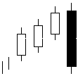
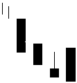
Examples

Bollinger Patterns

                Click on links to see some example patterns,

                Cup and handle Pattern
            

Example:

Description:

                An oscillator used to determine turning points, developed by
                John F. Ehlers.

                The Center of Gravity indicator was introduced by John F Ehlers
                in the May 2002 issue of Technical Analysis of Stocks and
                Commodities. Based on his worked with adaptive filters, Ehlers
                described the indicator as a unique new oscillator that it is
                smoothed and has essentially zero lag. The smoothing enables
                clear identification of turning points, and the zero lag aspect
                means action can be taken early in the move.

                Formula:

                COG = -1 * NUM / DEN

                n
                NUM  =          [ PRICE[i] * (i + 1) ]
                i = 0

                n
                DEN  =           PRICE[i]
                i = 0

                Where...
                PRICE[i] = The price of the ith bar back.
                PRICE[0] = price of current bar.
                PRICE[2] = price 2 bars back, etc.

                Essentially the numerator calculates a weighted sum of price
                while the numerator calculates the sum of price and the ratio
                represents the strength of movement in one direction.

            

Amazon: Rocket Science for Traders By John F. Ehlers

Example:

Description:

                Typical of most volatility measures, Chaikin's Volatility
                measures the separation between the high and low price of a
                stock. Specifically, Chaikin's Volatility uses the difference
                between current day average of the high and low and the average
                of the high and low, divided by the average high and low
                separation. Interpretations of this indicator involve watching
                for high volatility to indicate market peaks with low
                volatility possibly indicating a market bottom.

                The Chaikin Volatility indicator is the rate of change of the trading range.
                The indicator defines volatility as a increasing of the difference between
                the high and low. A rapid increases in the Chaikin Volatility indicate that
                a bottom is approaching. A slow decrease in the Chaikin Volatility indicates
                that a top is approaching.

                Formula:
            

Example:

Description:

Learn More

Learn More

                January 94 issue of Stocks & Commodities magazine

                Inspired by the prior work of Joe Granville and Larry Williams,
                Marc Chaikin developed a new volume indicator, extending the work
                done by his predecessors. The Chaikin Oscillator is a moving average
                oscillator based on the Accumulation/Distribution indicator.


                Interpretation


                The following discussion of volume accumulation/distribution
                interpretation, written by Marc Chaikin, is reprinted here with
                his permission:


                Technical analysis of both market averages and individual stocks must
                include volume studies in order to give the technician a true
                picture of the internal dynamics of a given market. Volume analysis
                helps in identifying internal strengths and weaknesses that exist
                under the cover of price action. Very often, volume divergences versus
                price movement are the only clues to an important reversal that is
                about to take place. While volume has always been mentioned by
                technicians as important, little effective volume work was done
                until Joe Granville and Larry Williams began to look at volume
                versus price in the late 1960s in a more creative way.


                For many years it had been accepted that volume and price normally
                rose and fell together, but when this relationship changed, the
                price action should be examined for a possible change of trend.
                The Granville OBV concept which views the total volume on an up
                day as accumulation and the total volume on a down day as distribution
                is a decent one, but much too simplistic to be of value. The
                reason is that there are too many important tops and bottoms,
                both short-term and intermediate-term, where OBV confirms the
                price extreme. However, when an OBV line gives a divergence signal
                versus a price extreme, it can be a valuable technical signal and
                usually triggers a reversal in price.

                Larry Williams took the OBV concept and improved on it. In order to
                determine whether there was accumulation or distribution in the
                market or an individual stock on a given day, Granville compared
                the closing price to the previous close, whereas Williams compared
                the closing price to the opening price. He [Williams] created a
                cumulative line by adding a percentage of total volume to the line
                if the close was higher than the opening and, subtracting a
                percentage of the total volume if the close was lower than its
                opening price. The accumulation/distribution line improved results
                dramatically over the classic OBV approach to volume divergences.

                Williams then took this one step further in analyzing the Dow Jones
                Industrials by creating an oscillator of the accumulation/distribution
                line for even better buy and sell signals. In the early 1970s,
                however, the opening price for stocks was eliminated from the daily
                newspaper and Williams' formula became difficult to compute without
                many daily calls to a stockbroker with a quote machine. Because of
                this void, I created the Chaikin Oscillator substituting the average
                price of the day for Williams' opening and took the approach one
                step further by applying the oscillator to stocks and commodities.
                The Chaikin Oscillator is an excellent tool for generating buy and
                sell signals when its action is compared to price movement. I
                believe it is a significant improvement over the work that preceded
                it.

                The premise behind my oscillator is three-fold. The first premise
                is that if a stock or market average closes above its midpoint for
                the day (as defined by [high + low] / 2), then there was accumulation
                on that day. The closer a stock or average closes to its high, the
                more accumulation there was. Conversely, if a stock closes below
                its midpoint for the day, there was distribution on that day.
                The closer a stock closes to its low, the more distribution there
                was.

                The second premise is that a healthy advance is accompanied by
                rising volume and a strong volume accumulation. Since volume is
                the fuel that powers rallies, it follows that lagging volume on
                rallies is a sign of less fuel available to move stocks higher.

                Conversely, declines are usually accompanied by low volume, but
                end with panic-like liquidation on the part of institutional
                investors. Thus, we look for a pickup in volume and then lower-lows
                on reduced volume with some accumulation before a valid bottom can
                develop.

                The third premise is that by using the Chaikin Oscillator, you can
                monitor the flow of volume into and out of the market. Comparing
                this flow to price action can help identify tops and bottoms,
                both short-term and intermediate-term.

                Since no technical approach works all the time, I suggest using
                the oscillator along with other technical indicators to avoid
                problems. I favor using a price envelope around a 21-day moving
                average and an overbought/oversold oscillator together with the
                Chaikin Oscillator for the best short and intermediate-term technical
                signals.

                The most important signal generated by the Chaikin Oscillator
                occurs when prices reach a new high or new low for a swing,
                particularly at an overbought or oversold level, and the oscillator
                fails to exceed its previous extreme reading and then reverses
                direction.

                1. Signals in the direction of the intermediate-term trend are
                more reliable than those against the trend.

                2. A confirmed high or low does not imply any further price
                action in that direction. I view that as a non-event.

                A second way to use the Chaikin Oscillator is to view a change of
                direction in the oscillator as a buy or sell signal, but only in
                the direction of the trend. For example, if we say that a stock
                that is above its 90-day moving average of price is in an uptrend,
                then an upturn of the oscillator while in negative territory would
                constitute a buy signal only if the stock were above its 90-day
                moving average--not below it.

                A downturn of the oscillator while in positive territory (above zero)
                would be a sell signal if the stock were below its 90-day moving
                average of closing prices.

                Formula:

                The Chaikin Oscillator is created by subtracting a 10-period
                exponential moving average of the Accumulation/Distribution
                Line from a 3-period exponential moving average of the
                Accumulation/Distribution Line.


            

Example:

Description:

                The Chandelier Exit is a volatility
                measure using the ATR to help set stop limits. The exit is
                computed by finding the highest value over the period and then
                subtracting a multiple of the ATR for that period. On
                StockFetcher, the position parameter is the ATR multiplier
                used to find the actual stop position.
            

Amazon: Technical Traders Guide to Computer Analysis of the Futures Markets By Charles Lebeau

Example:

Description:

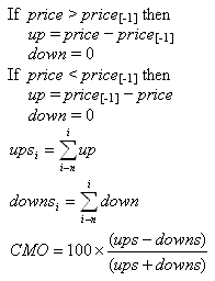
                The Chande Momentum Oscillator (CMO) was developed by Tushar Chande.
                A scientist, an inventor, and a respected trading system developer,
                Mr. Chande developed the CMO to capture what he calls pure momentum".
                For more definitive information on the CMO and other indicators we
                highly recommend the book The New Technical Trader by Tushar Chande
                and Stanley Kroll.

                The CMO is closely related to, yet unique from, other momentum
                oriented indicators such as Relative Strength Index, Stochastic,
                Rate-of-Change, etc. It is most closely related to Welles Wilders
                RSI, yet it differs in several ways:

                • It uses data for both up days and down days in the numerator,
                thereby directly measuring momentum.

                • The calculations are applied on unsmoothed data. Therefore,
                short-term extreme movements in price are not hidden. Once
                calculated, smoothing can be applied to the CMO, if desired.

                • The scale is bounded between +100 and -100, thereby allowing
                you to clearly see changes in net momentum using the 0 level.
                The bounded scale also allows you to conveniently compare
                values across different securities.

                Interpretation

                The CMO can be used to measure several conditions.

                Overbought/oversold: The primary method of interpreting the CMO
                is looking for extreme overbought and oversold conditions. As a
                general rule, Mr. Chande quantifies an overbought level at +50 and
                the oversold level at -50.  At +50, up-day momentum is three times
                the down-day momentum. Likewise, at -50, down-day momentum is three
                times the up-day momentum.  These levels correspond to the 70/30
                levels on the RSI indicator.

                You could also establish overbought/oversold entry and exit rules
                by plotting a moving average trigger line on the CMO. For example,
                if you are using the default 20-period CMO, a 9-period moving
                average may serve as a good trigger line. Buy when the CMO crosses
                above the 9-period trigger line; sell when it crosses below.

                Trendiness: The CMO (much like the VHF indicator), can also be
                used to measure the degree to which a security is trending. The
                higher the CMO, the stronger the trend. Low values of the CMO
                show a security in a sideways trading range.

                You may find the CMO helpful in establishing the entry and exit
                rules of a trend following system. Enter when the CMO is high and
                exit when it moves lower.

                Divergence.  Although not specifically mentioned in Mr. Chandes
                book, you could also look for divergence between the CMO and the
                price, as is often done with other momentum indicators. See the
                discussion about divergence in the Interpretation section of RSI.

                Other: Although not specifically mentioned in Mr. Chandes book,
                you may also look for chart formations (head and shoulders, rising
                wedges, etc.), failure swings, and support/resistance.  See the
                discussion on these methods in the Interpretation section of RSI.
            

Amazon: The New Technical Trader By Tushar S. Chande

Example:

Description:

                A very specific phrase, the channel phrase allows a user to
                search for stocks that are trading within some computed
                boundaries.

                Outside of just identifying stocks which are
                trading within a channel, this phrase can allow a user to look
                for stocks specifically trading near the top or bottom of the
                channel.

                Finally, the channel does not have to be flat, but
                could actually have a positive or negative slope by using the
                increasing or decreasing keywords.
                
                Channel Analysis, beginning on page 18 of the 
                July 1998 Technical Analysis of Stocks and Commodities Magazine 
            

Example:

Description:

                chart color customization page. While this is by no means
                polished, we thought it would provide immediate benefit for
                a number of StockFetcher members.

            

Chart Color

Example:

Description:

                chart-display is a very specific phrase that tells a chart to be
                to weekly mode. Like the other chart options, this does not affect
                screening results; instead it provides another way to draw the chart.
                By telling StockFetcher to place the chart in weekly mode, all of
                the plots, invluding price are converted to the appropriate weekly
                values. Any measuers or indicators that were a part of th screen are
                also converted to their weekly conterpart. As an example below is a
                screen that look for a 10 and 50 day moving average cross over.

                Adding the phrase chart-display is weekly to this screen doesn't
                affect the individual  matches; however, it does convert our
                averages from 10 and 50 day to 10 and 50 week averages.

                While providing the ability to analyze charts, this addition can be
                confiusion when cerifying that a particular condition occurred.
                Therefore, it is important to be careful using weekly charts.
            

Example:

Description:

                As with other available charting tools, changing the scale from linear to logarithmic is an
                important feature on StockFetcher. Analyzing price information on a logarithmic scale can
                smooth some of the edges found when viewing long-term plots spanning a large price range. On
                StockFetcher, changing the scale of the chart can either be accomplished from the Chart Settings
                section, or through the phrase chart-scale is. The two scale options available are linear
                and logarithmic. Below is an example illustrating this phrase.

                By default StockFetcher displays charts using the linear scaling.

                Chart-scale is only applied to the primary (price) plot. Other
                plots, such as volume, MACD, RSI, etc, are always linear.
            

Example:

Description:

                Chart-size tells StockFetcher how wide the resulting charts should
                be. This is entirely a user preference when it comes to analyzing
                charts, as well as managing bandwidth. Available widths include:

                Possible Values:
                • Small
                • Medium
                • Large
                • Giant
                • Huge
                • 100 to 1024

                In addition, specific pixel values of 100 to 1024 may be specified
                for the chart-width.
            

Example:

Description:

                As with any stock chart package, changing the amount of time covered
                by a chart on StockFetcher is critical. By default, StockFetcher
                provides 3-month, 6-month, and 1 year plot periods. Using the
                chart-time key phrase it is possible to customize the default time
                period for the charts. The chart-time may be configured from 2 years
                down to single day plots.

                While a single day plot typically doesn't provide much perspective,
                short-term charts can provide important details when researching
                recent price or measure activity. For example, the detailed screen
                below watches for two crossovers in a short period of time. Reducing
                the amount of time for the plot allows for greater inspection of
                the activity.

                MA(10) 5 days ago crossed above the MA(50) 5 days ago
                and MA(10) 1 day ago has been above
                and the MA(50) 1 day ago for 3 days
                and MA(10) is below the MA(50) and Chart-time is 2 weeks

                The moving average analysis above describes a specific double
                crossover, but further information about the strength of the first
                crossover is easily seen in the resulting charts.
            

Example:

Description:

                Chart-type can be used to force the charts to draw the price
                values in a specific way, overriding StockFetcher's default
                rules.
            

Example:

Description:

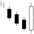
                The chart-type option directs StockFetcher to change the default
                plotting style for stock prices. The available chart-types are
                line, OHLC and candlestick. The line option simply displays the
                price using a single value, the close. The OHLC option plots all
                4 fundamental values.

                The lowest value on the bar represents the low, the tick facing
                left is the open, the tick facing right is the close, and the
                tallest point is the high. The following is an examples of an
                OHLC chart.

                Finally the candlestick plot type is a popular short-term
                plotting style. Again including all 4 price values, the
                candlestick has 4 main characteristics.

                •   the tail, which ends at the lowest value of the day

                •   the body, represents the range covered by the
                high and low

                •   the head, ends at the high of the day

                •   the body color, a shaded body indicates a close
                below the low while a clear or white body
                indicates an increase in the price from open to close.

                Depending on the timeframe used for charts, the chart-type can
                either simplify the chart viewing, or provide additional
                information for making decisions about the price pattern of a
                stock.

                Below are a couple examples demonstrating how to change the
                default chart-type:

                Close is below the lower Bollinger band
                and Chart-time is 1 year and Chart-type is line


                High is above high 1 day ago
                and Low is below low 1 day ago
                Depending on the timeframe used for charts, the chart-type can
                either simplify the chart viewing, or provide additional
                information for making decisions about the price pattern of a
                stock.

                Below are a couple examples demonstrating how to change the
                default chart-type:

                Close is below the lower Bollinger band
                and Chart-time is 1 year and Chart-type is line


                High is above high 1 day ago
                and Low is below low 1 day ago
                and Chart-time is 2 months
                and Chart-type is candlestick

                The above provide excellent examples of where the actual price
                charting style can greatly enhance the interpretation of a chart
            

Example:

Description:

                The Close-to-open gap is a simple measure of a stock's opening
                price relative the previous close. The resulting values from
                this measure are the difference between the open and close
                represented as a percent of the closing price.
            

Example:

Description:

                By default, StockFetcher returns basic price and volume information
                for each of the stocks returned in a screen.

                This information includes:

                • most recent closing price.
                • percent change from previous close.
                • the number of shares traded during the most
                recent day.

                The results columns can easily be augmented using the add column
                phrase. With add column nearly any measure or indicator may be added
                to the filter results. As an example, the ten day average volume is
                added as a column to a basic stock screen:

                Price is between 10 and 50
                and Add column average volume(10)

                Now the results present the ten day average volume along with the
                standard information.

                In addition to providing new information with the filter results,
                each new measure can be sorted in either ascending or descending
                order by clicking on the appropriate column header. Sorting these
                additional columns is useful with measures whose high or low values
                can provide additional approach confirmation. For example, take an
                approach where the close-to-open gap in price is displayed.

                Show stocks where the price is between 10 and 15
                and Add column close to open gap

                Clicking on the column heading for the "close to open gap"
                immediately presents the results where the most recent open price
                gapped significantly from the closing price the day before.

                Column Aliases

                Enclosing text inside the {} symbols provides an optional extension
                to the "add column" phrase. These braces are used to rename
                resulting column headers to something more concise or meaningful.
                Taking the average volume example above, suppose the column is
                renamed to "av10" to clean up the results.

                Price is between 10 and 50
                and Add column average volume(10) {av10}

                The contents inside the {...} will be used as the new column header.
                This extension definitely proves useful when many measures are added
                to the results, or when the actual measures added to the results
                are complex and produce difficult to read headers. In the example
                below, a 52-week high of the MA(50) is added to the results.

                Price is between 10 and 50
                and Add column average volume(10) {av10}
                and Add column MA(50) 52 week high {ma50hi}
            

Example:

Description:

Learn More

                The Commodity Channel Index ("CCI") measures the variation of a
                security's price from its statistical mean. High values show that
                prices are unusually high compared to average prices whereas low
                values indicate that prices are unusually low. Contrary to its name,
                the CCI can be used effectively on any type of security, not
                just commodities.

                Interpretation

                There are two basic methods of interpreting the CCI: looking for
                divergences and as an overbought/oversold indicator.

                • A divergence occurs when the security's prices are making
                new highs while the CCI is failing to surpass its previous highs.
                This classic divergence is usually followed by a correction in
                the security's price.

                • The CCI typically oscillates between 100. To use the CCI
                as an overbought/oversold indicator, readings above +100 imply
                an overbought condition (and a pending price correction) while
                readings below -100 imply an oversold condition (and a pending
                rally).

                Further details on the contents and interpretation of the CCI can
                be found in an article by Donald Lambert that appeared in the
                October 1980 issue of Commodities (now known as Futures) Magazine.

                Formula:

                A complete explanation of the CCI calculation is beyond the scope
                of this document. The following are basic steps involved in the calculation:

                1. Add each period's high, low, and close and divide this sum by 3.
                This is the typical price.

                2. Calculate an n-period simple moving average of the typical prices
                computed in Step 1.

                3. For each of the prior n-periods, subtract today's Step 2 value
                from Step 1's value n days ago. For example, if you were
                calculating a 5-day CCI, you would perform five subtractions
                using today's Step 2 value.

                4. Calculate an n-period simple moving average of the absolute values
                of each of the results in Step 3.

                5. Multiply the value in Step 4 by 0.015.

                6. Subtract the value from Step 2 from the value in Step 1.

                7. Divide the value in Step 6 by the value in Step 5.
            

Example:

Description:

                The comparative relative strength performs a simple calculation
                of how a stock performed, over the specified period of time,
                with a given input stock. This measure is often used to find
                stocks that are underperforming or outperforming a given index,
                but can also be used to compare against individual stocks. It
                should be noted that this measure is not a pattern matching
                routine. That is, it simply looks to see the price change from
                beginning to end, not what happened in the middle. All values
                above 1.0 indicate that a stock has outperformed the input
                stock, where any value below 1.0 indicates
                underperformance.

            

Example:

Description:

                When evaluating screen results, it can be helpful to compare the
                results with a known "good" stock. The comparison chart feature
                allows you to view the price change comparison between any
                of your filter matches and a given stock.

                As an example, suppose you are interested in stocks that
                recently had a moving average crossover, but you would also
                like to visually compare any matches with the Nasdaq Composite.

                Show stocks where the MA(10) crossed above the MA(50)
                and draw comparison chart(^IXIC)


            

Example:

Description:

                count As a basic example, suppose you are interested in stocks
                that have set multiple 1 year highs over the last 30 days:

                Current Limitations:

                • You can only include a single screen within the
                count(...) text. That is, you can't include filters
                which have been joined with "and" inside of the
                count(...) text.

                • There is a limit of 100 days for accumulating the
                counts. This restriction is based on performance and
                hopefully we will be able to increase that value.
            

Example:

Description:

Learn More

                Custom exponential moving averages CEMA In addition to creating
                custom simple moving averages, you can now create your own
                custom exponential moving averages (CEMA) and custom weighted
                moving averages (CWMA). The usage is the same as the custom
                moving average (CMA).

                EMA Formula:
            

                WMA Formula:
            

Example:

Description:

Learn More

                You can create your own custom moving averages for any measure
                on StockFetcher. The moving average is based on the simple
                moving average forumula. At this time we do not support custom
                exponential moving averages.

                Formula:
            

Example:

Description:

Learn More

                Description
                The Darvas trading technique is designed as a method of capturing the
                strength of the trend. The buy signals are generated on new bullish
                strength and managed by using the five day volatility range to set a
                stop loss.

                The Darvas approach is built around long term trend trading. It is a
                bullish approach that is most suited to trending stocks, and also to
                trending markets. Darvas was able to follow and trade stocks without
                the need for intra day prices, or to be constantly in front of a screen,
                or even to have access to daily prices. This makes the approach
                particularly useful for readers who have full time jobs. Darvas
                applies a filter - a Darvas box (DB) - to price movements to help
                determine which price moves are significant, and which are not. The
                filter is established by upper and lower limits of a Darvas box.


                The top of the Darvas box always starts with a new high. This high
                must be followed by 3 days that are lower. The bottom of the Darvas
                box can only be calculated after the top of the Darvas box has been
                confirmed. It is constructed in the opposite way to the top of the
                box. It uses as its starting point the lowest low that occurs AFTER
                the top of the Darvas box is established. It is again a 4 day pattern,
                but it starts 1 day after the top of the box pattern. This means it
                takes a minimum of 5 days for a Darvas box to be identified for both
                top and bottom.

                From:

            

Amazon: Nicolas Darvas book, How I Made $2,000,000 in the Stock Market

Example:

Description:

                At a first glance the term date offset would be covered by the
                days ago phrasing. But, there is an important difference between
                the two constructs. days ago is important when creating a
                specific trading approach; it permits access to historical
                prices or measures for generating screens. "Date offset" is very
                different from this. In essence date offset is used to back test
                an entire screening approach. By specifying a date offset in the
                filter text indicates to StockFetcher that the entire screening
                approach needs to be run from a particular date in the past.

                The date offset provides an essential tool not only for judging
                the performance of a particular approach from different dates
                in the past, but it also helps to verify the quantity and
                quality of matches produced by an approach. Some approaches may
                produce more or less matches based on the market conditions at
                that time. Using the date offset helps to establish whether or
                not an approach is easily swayed by a changing environment.

                Using the date offset phrasing is very simple. All that is
                required is the text date offset along with a number of days.
                Below is an approach that returns matches ten days prior to the
                current date:

                RSI(14) crossed above 30 and date offset is 10

                Date offsets of as little as a single day and up to 1 year are
                valid on StockFetcher.

                Mentioned above, the date offset is not related to the days ago
                phrasing. An approach using days ago uses a look-back for the
                specific measure(s) involved. Including a date offset increases
                the number of days used in the days ago phrase.

                Once the offset has been applied to a screen, StockFetcher
                provides additional results that help to analyze the performance
                of a screen. From the results page, it is possible to see the
                price change from the offset specified to the current date.
                Additionally, accessing the performance pop-up provides
                breakdowns of different time periods as well as more information
                about advancing and declining matches. For U.S. stocks, the
                performance window also returns the performance of the major
                indices to help judge the matches' performance.
            

Example:

Description:

                This is a simple measure of the difference (in percent) of the
                most recent closing prices of a stock. The absolute day change
                disregards the sign of the change, so the results indicate the
                magnitude of the change.
            

Example:

Description:

                The Day Position is a basic measure that computes a value which
                is a percentage of the day range. In otherwords, if the
                position parameter is 0.5, the Day Position will be
                Low + ((High - Low) * 0.5). Any value from 0 to 1 may be used
                to locate a position within the daily range.

                In addition to computing this value over a single day, a period
                may be specified. The measure will then find the highest high
                and lowest low over the given number of days and then perform
                the same computation as above.

                Note: By default the day position

                Example 1. Finds stocks where the close was in the top half of
                the trading range for the day:

                Example 2. Finds stocks where the open was in the lower quarter
                of the trading range for the last 1 week

Example:

Description:

                The day range returns the difference between the high and low
                prices of the day, represented as a percent of the closing
                value. For example, suppose a stock closed at 10, the high was
                11 and the low was 9. The difference between the high and low
                is 2. Represented as a percent, the day range is: 20%.

                The average day range computes a simple average of the day range
                over a given number of days. This value is also represented as
                a percent of the closing price.

                Finally, the day point range is the actual price difference
                between the high and low of the day. The day point range is
                not converted to a percent.

Example:

Description:

                Nearly all screening approaches require the ability to specify a
                value or values from the past. This could include a single
                price, a volume change, the position of an oscillator, or the
                entire range of an indicator from some specified offset.
                Through the construction of phrases using days/weeks/months
                ago, StockFetcher permits access to nearly any value in the
                past.

                While this feature is not limited to price values from
                only one or two days ago, it is just that ability that allows
                for creating classic and custom candlestick patterns. The first
                example shows an outside reversal, using the offset phrasing.

                High is above high 1 day ago and Low is below low 1 day ago and
                Close is above Open and Close 1 day ago is below Open 1 day ago

                The example demonstrates a very straightforward and logical
                way to refer to specific values from just 1 day ago. Notice
                that any time an offset is required it must immediately follow
                the measure it refers to. The offset is not carried through to
                any specific value. While this property may result in longer
                phrases, it allows complete control of a screening approach.

                For another example using the offset, suppose a trading
                approach requires that the MACD histogram had been increasing
                for 5 successive days up until the last couple of days.

                MACD Histogram(12,26,9) 2 days ago had been increasing for 5 days
                and MACD Histogram(12,26,9) has been decreasing for 2 days

                By simply changing the offset of the MACD Histogram reference, in
                conjunction with the increasing and decreasing keywords, the
                approach above discovers a local maximum. No pattern is safe
                from being detected using the "days ago" phrasing on
                StockFetcher!

                The offset phrasing also helps in avoiding a
                critical flaw that affects many approaches where a measure
                crosses a simple moving average. In this case, an example
                screen detecting a spike in daily shares traded is used.
                Suppose the approach looks for a 50% increase in the shares
                traded versus the 10-day average of shares.

                Volume is more than 50% above the average volume(10)

                The approach above works and will return valid match, but the
                approach is flawed and does not return all of the symbols possible.
                The mistake is that the 10-day average volume includes the unusual volume
                spike. With StockFetcher, it is very easy to solve this
                problem:

                Volume is more than 50% above the average volume(10) 1
                day ago

                Advanced Examples The true power of the "... days ago"
                key phrase can be seen when it comes to defining specific
                patterns with a particular measure or a stocks price. For
                example, take the case where the price of a stock dips below
                the lower Bollinger Band, remains in that position for a couple
                of days and has just started to leave the band. This entire
                pattern may be described using combinations of the offset pattern.

                High 5 days ago crossed below the lower Bollinger(20)
                and High1 day ago had been below the lower Bollinger(20)
                for 4 days
                and Low is above the lower Bollinger(20)

                The screen above defines an exact pattern than can easily be
                verified from the charts.
            

Example:

Description:

                a new filter construct that allows you to filter based on the number
                of days since a particular event occurs. The "days" feature allows
                you to specify the event and a period of time; it returns the number
                of days since the event most recently occurred.

                For example, suppose you want to find stocks where the most recent
                Bollinger breach was 10 days ago:

                show stocks where days(high above upper Bollinger(20),15)
                equals 10


                Another example that controls the timing of two moving average
                crossovers:

                show stocks where the days(MA(10) crossed below MA(50),30) is
                above 20 and days(MA(10) crossed above MA(50),20) is above 0


                Finally, an example where the 14-day RSI crossed from below 30 to
                above 70 within the last 2 weeks:

                show stocks where days(RSI(14) crossed above 30,10) is above
                days(RSI(14) crossed above 70,10)
                and days(RSI(14) crossed above 70,10) is above -1


                Note: the "above -1" portion of the filter adds the requirement that
                the crossover above 70 must have occurred.

            

Example:

Description:

               Developed by Thomas R. Demark, this indicator attempts to detect 
               price tops and bottoms through adjacent highs and lows.

               First, an average of differences is computed from the current intraday 
               high and previous intraday high. If the current high is above the 
               previous, the difference is used, otherwise nothing is added. Next, 
               the same process is used for current intraday lows which are less than 
               the previous intraday low. Finally, a ratio is computed by taking the 
               average of highs over the sum of the average high and low differences.

               The DeMarker values range between 0 and 1.0 with 0.30 and 0.70 considered 
               to be important thresholds. 
            

               Demarker Technical Indicator is based on the comparison of the period 
               maximum with the previous period maximum. If the current period (bar) 
               maximum is higher, the respective difference between the two will be 
               registered. If the current maximum is lower or equaling the maximum of 
               the previous period, the naught value will be registered. The differences 
               received for N periods are then summarized. The received value is used as 
               the numerator of the DeMarker and will be divided by the same value plus 
               the sum of differences between the price minima of the previous and the 
               current periods (bars). If the current price minimum is greater than that 
               of the previous bar, the naught value will be registered.

               When the indicator falls below 30, the bullish price reversal should be 
               expected. When the indicator rises above 70, the bearish price reversal 
               should be expected.

               If you use periods of longer duration, when calculating the indicator,
               you'll be able to catch the long term market tendency. Indicators based on 
               short periods let you enter the market at the point of the least risk and plan 
               the time of transaction so that it falls in with the major trend.


             Calculation:

             Parameters:

               1. N - time period.

            Calculation:

            The value of the demarker for the j-th interval is calculated as follows:

               1. The DeMaxj is calculated.
                  If   highj > highj-1  , then  DeMaxj = highj - highj-1  , otherwise  DeMaxj = 0
               2. The DeMinj is calculated.
                  If  lowj < lowj-1 , then  DeMinj = lowj-1 - lowj , otherwise  DeMinj = 0
               3. The value of the demarker is calculated as:
              
            

Amazon: Thomas Demark book The New Science of Technical Analysis

Example:

Description:

                The Detrended Price Oscillator (DPO) computes the difference
                between the current closing value of a stock and a specified
                moving average. The basic idea behind the DPO is to detect
                cycles in stocks as opposed to trends.

                Formula:

                To calculate the Detrended Price Oscillator, first create an
                n-period simple moving average (where "n" is the number of
                periods in the moving average).
            

                Now, subtract the moving average "(n / 2) + 1" days ago, from
                the closing price. The result is the DPO.
            

Example:

Description:

Learn More

                The DI was developed by J. Welles Wilder and is described in his
                1978 book New Concepts In Technical Trading Systems.

                The Directional Movement System helps determine if a security is
                "trending." It was developed by Welles Wilder and is explained in
                his book, New Concepts in Technical Trading Systems.

                Interpretation

                The basic Directional Movement trading system involves comparing
                the 14-day +DI ("Directional Indicator") and the 14-day -DI. This
                can be done by plotting the two indicators on top of each other
                or by subtracting the +DI from the -DI. Wilder suggests buying
                when the +DI rises above the -DI and selling when the +DI falls
                below the -DI.

                Wilder qualifies these simple trading rules with the "extreme
                point rule." This rule is designed to prevent whipsaws and reduce
                the number of trades. The extreme point rule requires that on
                the day that the +DI and -DI cross, you note the "extreme point."
                When the +DI rises above the -DI, the extreme price is the high
                price on the day the lines cross. When the +DI falls below the -DI,
                the extreme price is the low price on the day the lines cross.

                The extreme point is then used as a trigger point at which you
                should implement the trade. For example, after receiving a buy
                signal (the +DI rose above the -DI), you should then wait until
                the security's price rises above the extreme point (the high price
                on the day that the +DI and -DI lines crossed) before buying. If
                the price fails to rise above the extreme point, you should continue
                to hold your short position.

                In Wilder's book, he notes that this system works best on securities
                that have a high Commodity Selection Index. He says, "as a rule of
                thumb, the system will be profitable on commodities that have a
                CSI value above 25. When the CSI drops below 20, then do not use
                a trend-following system."

                Formula:
            

Amazon: New Concepts in Technical Trading System by J. Welles Wilder

Example:

Description:

                There are 3 dividend related measures. These include:

                • annual dividend per share
                • dividend yield
                • days since last dividend
            

Example:

Description:

                Donchian Channels, created by Richard Donchian [Donchian ???],
                are envelopes around the price based on the highest and lowest
                prices during the given number of days. The center band is
                computed by taking the average of the upper and lower band.
                These bands can be used to find potential areas of support and
                resistance based on recent price activity. StockFetcher allows
                a second parameter to the Donchian Channels that indicates a
                lag or offset used in the computation. This lag is used to
                offset the period of time for finding the highest and lowest
                values. For example if "5" is used as the lag parameter and
                "20" is used as the period, then the highest and lowest values
                are discovered from the 20 days of history which started 5
                days in the past. When lag is used, it is possible to have
                recent price values which exceed the upper or lower band.
                Without lag, the Donchian Channels will always contain all of
                the prices within the specified period.
            

Example:

Description:

                The syntax is the same as the "draw" command, with the exception
                of the preceding "do not".

                *Notes*
                • In the case of indicators that produce multiple lines
                (i.e. MACD, Stochastics, Bollinger Bands) you can not remove
                specific lines. The "do not draw" will remove all of the lines
                for those specific measures.

                • At the current time it is not possible to remove the
                volume plot.
            

Example:

Description:

                pattern detector attempts to discover stocks that are nearing or
                have recently completed a double-bottom. Below is an example
                screen using this new pattern:

                Please note the - (hyphen) in double-bottom, that is required to
                produce the correct results.

                As background, to meet the requirements of this pattern, the
                following conditions must be met:

                • Stock is in a recent downtrend
                • Retracement of more than 10% of the low after the downtrend.
                • Return to within 3% of the lower resistance
                • Retest of the upper resistance
                • Increase of volume on the retest of upper resistance.

                Below is a chart demonstrating these qualifications:
            

                Please keep in mind this is a fairly specific implementation of
                the double-bottom and may yield very few results each day.
                Additionally, we will continue to analyze the results, so if
                you have any ideas or suggestions for this pattern, please
                don't hesitate to drop us a line!

                By default the double-bottom algorithm will look for matches that
                broke resistance within the last 6 trading days. To modify that,
                you can add a parameter to the double bottom. For example:

                1. pattern is double-bottom(25) and price is above 2

                2. pattern is double-bottom(3) and price is above 2


                The first example will look for double-bottoms that completed
                within the last 25 trading days, and the second looks for very
                recent ones.

                To learn more about how this feature works, check out the post in
                the announcements section of the forums:

            

                Technical Nerd Note:

                I am not sure why but when you try and add a comlumn that uses
                "double-bottom" or "incomplete double-bottom(PERIOD)" it does
                not work. But if you use "dt" or "dt2" then you get a strange
                column heading (MISCPATS?MODE=4 & MISCPATS?MODE=3) and a 
                1.0 if pattern is correct or "-99999997952.00" if the pattern
                is not a double top. That is probably a small glimpse inside how
                SF works. MISCPATS might stand for "Misc Paterns" and mode may be
                the index of the given pattern.

            

Example:

Description:

                Draw lines based up measure or variable values.

                you can draw lines based upon measure values.

                Note: this is only a cosmetic feature, it does not effect filter
                results.

                Examples:

                1. Draw lines based on price values.

                show stocks where MA(10) crossed above MA(50)
                and draw price line at high
                and draw price line at low


                2. Draw lines based on previous values of a measure.

                show stocks where the RSI(14) is above 70
                and draw RSI(14) line at RSI(14) 1 day ago


                3. Create custom channels based on a measure.

                set{myhigh,high 60 day high}
                set{mylow, low 60 day low}
                set{upper,myhigh * 0.99}
                set{lower,mylow * 1.01}
                show stocks where MA(10) crossed above MA(50)
                and draw price line at upper
                and draw price line at lower



                4. And one last example:

                show stocks where low crossed above upper Bollinger Band(20)
                and draw price line at Upper Bollinger Band(20)
                and draw price line at Lower Bollinger Band(20)
            

Example:

Description:

                on plot - You can direct your draw commands to specific plots.
                The usage for this new feature is:

                draw [MEASURE] on plot [MEASURE]

                you can not directly draw a basic price value (open, high, low,
                close) on a different plot. You will want to assign these to
                variables first.


                StockFetcher automatically plots the appropriate measures
                included in a screening approach. However, plotting additional
                measures, not a part of the stock screen, can be extremely
                helpful to the analysis process. Nearly any number of additional
                measures may be plotted through the draw keyword. The strength
                of adding charted measures is the ability to confirm a trading
                approach, as well as further develop and refine an approach. As
                an example, take a basic approach of selecting stocks breaking
                through the lower Bollinger Band.

                Close is below the lower Bollinger band(20)

                The above is an easy test to find stocks trading below a
                statistical lower bound. Browsing through the results reveals a
                large number of choices, with very diverse characteristics.

                After viewing a few charts, it becomes apparent that this
                approach could be strengthened by finding stocks that were in a
                long-term positive trend prior to the current down trend.
                However, suppose the actual method of determining this longer
                trend is not available. To help develop the trend detection, a
                200-day moving average is added to the charts.

                Close is below the lower Bollinger band(20)
                And draw MA(200)

                This new addition will not affect the total number of matches
                from the first part of the filter.

                After reviewing the charts with this new information, it is much
                easier to locate, from chart analysis, stocks in a strong
                uptrend. Simply including a plot of the MA(200) on the charts
                provides a simple and quick chart-based screening mechanism.

                The draw command may be used to add any number of measures and
                indicators to plots and is not limited to any particular
                measures. As noted above, the draw command will not affect the
                filter output. Additionally, duplicate instances of the same
                measure will not be a problem in cases where a screen includes
                the same measure as a draw command. draw options may be accessed
                by manually entering the text when creating a filter, or by
                saving the options in the Chart Settings section.
            

Example:

Description:

                The Ease of Movement indicator shows the relationship between
                volume and price change. As with Equivolume charting, this indicator
                shows how much volume is required to move prices.

                The Ease of Movement indicator was developed Richard W. Arms, Jr.,
                the creator of Equivolume.

                Interpretation

                High Ease of Movement values occur when prices are moving upward
                on light volume. Low Ease of Movement values occur when prices are
                moving downward on light volume. If prices are not moving, or if
                heavy volume is required to move prices, then the indicator will
                also be near zero.

                The Ease of Movement indicator produces a buy signal when it
                crosses above zero, indicating that prices are moving upward more
                easily; a sell signal is given when the indicator crosses below
                zero, indicating that prices are moving downward more easily.

                Formula:

                To calculate the Ease of Movement indicator, first calculate the
                Midpoint Move as shown below.
            

                Next, calculate the "High-Low" Box Ratio expressed in eighths with
                the denominator dropped (e.g., 1-1/2 points = 12/8 or just 12).

            

                The Ease of Movement ("EMV") indicator is then calculated from
                the Midpoint Move and Box Ratio.

                The raw Ease of Movement value is usually smoothed with a moving
                average.

            

Example:

Description:

                Used to describe equality relationship input measures, values
                and time
            

                "within" symantics:

                The "within the last" is not supported with the "above" or
                "below" phrases. Typically "within the last" is allowed when a
                particular event occurs, such as a crossover.

                For example:

                MA(10) crossed above MA(50) within the last 5 days


                To use "within" type syntax for your example, you will want to
                use the "count()" feature. For example:

                show stocks where count(opcl% is above 30%,5) is above 0
                and price above 1

                The following example is an error:

                show stocks where the opcl% is above 30%
                within the last 5 days
                and price above 1

                This is a work around to produce the results:

                set{myOpclPrct, opcl%}
                set{myConst, 30}
                show stocks where myOpclPrct crossed above myConst
                within the last 2 days

                and price above 1
            

Example:

Description:

                Developed by William Blau, the Ergodic Candlestick Oscillator
                examines the average ratio of the day change versus the day's
                trading range. An n-day EMA of the close to open change is
                divided by an n-day EMA of the difference between the high and
                low. This ratio is then smoothed by a m-day EMA.

                There are two parameters used with the ECO on StockFetcher. The
                first indicates the period used for averaging the day change
                and day range. The second period specifies the period for the
                EMA used on the ratio of the day change and range.

                The basic idea behind this measure is that in cases where the
                stock is making positive net changes on large trading ranges,
                the ECO values will be positive. In cases where the stock is
                trading lower each day, the ECO will be negative.
            

Amazon: Momentum, Direction, and Divergence By William Blau

Example:

Description:

                The ERSI uses the values from an exponential moving average
                (EMA) as input to the RSI computation. On StockFetcher, the
                first parameter of the ERSI represents the period used for the
                RSI computation and the second parameter is the period of the
                EMA used as input. By using EMA values as input, the ERSI will
                be less volatile than the standard RSI.
            

Example:

Description:

                Also See "Market is"

                You can filter for Exchage by it's name or by it's number. See
                "Market is" for more details.

            

Example:

Description:

SEC: Learn More

WikiPedia: Learn More

                ETF is A fund that tracks an index, but can be traded like a stock.
                ETFs always bundle together the securities that are in an index;
                they never track actively managed mutual fund portfolios (because
                most actively managed funds only disclose their holdings a few
                times a year, so the ETF would not know when to adjust its holdings
                most of the time). Investors can do just about anything with an
                ETF that they can do with a normal stock, such as short selling.
                Because ETFs are traded on stock exchanges, they can be bought and
                sold at any time during the day (unlike most mutual funds). Their
                price will fluctuate from moment to moment, just like any other
                stock's price, and an investor will need a broker in order to
                purchase them, which means that he/she will have to pay a commission.
                On the plus side, ETFs are more tax-efficient than normal mutual
                funds, and since they track indexes they have very low operating
                and transaction costs associated with them. There are no sales
                loads or investment minimums required to purchase an ETF. The
                first ETF created was the Standard and Poor's Deposit Receipt
                (SPDR, pronounced "Spider") in 1993. SPDRs gave investors an easy
                way to track the S&P 500 without buying an index fund, and they
                soon become quite popular.
            

Amazon: The Exchange-Traded Funds Manual by Gary L. Gastineau

Example:

Description:

                see: Fibonacci Retracement Lines
                from: 1997 November TASC Traders Tip, by Thom Hartle
            

Example:

Description:

                The Fibonacci retracement lines are ranges computed from the
                high and low over a given period of time. The actual lines
                that are drawn are specific percent retracements from the
                given high or low. Investors primarily look at 3 different
                lines (0.382,0.50,0.618), which are based on the historical
                formula for the Fibonacci sequence.

                These Fibonacci retracements can occur both after a recent
                downturn or swing low; or after a run-up. The actual target
                values are computed by taking a percent change from the high
                or low value.

                By specifying Fibonacci Down on StockFetcher, you are referring
                to the retracement lines drawn after a recent swing low. All of
                the values will be relative to how much the stock has recovered
                from the recent low. For the Fibonacci Up, the values are
                based upon a recent run-up in the stock price. Again, the
                actual values refer to the amount the stock has moved to return
                to the recent low.

                Below is an example of the Fibonacci Down screen:
            

                The actual values returned by StockFetcher are computed from the
                most recent close in reference to the recent high or low. In
                the example above, the value returned by the screen wold be
                near 0.382 (the most recent close is very near the 0.382
                Fibonacci band.)

                Note: When spcecifying the Fibonacci Up, the values returned
                will be reversed from the Fibonacci Down. So a filter scanning
                for crossed above in the Fibonacci Up case will actually result
                in a downward price move.

                StockFetcher allows several parameters with the Fibonacci retracements.

                • time - The first parameter is the length of time used to look
                for the up-trend or down-trend. So, a value of 65 will search
                over the last 3 months to look for the trend.

                • min length - The second parameter is the minimum number of
                days for the trend to occur. For example, if you specify 15
                days here, that means the distance between the high and low
                must be at least 15 days.

                • labels on/off - Finally, by setting the third or last
                parameter to 0, you can eliminate the labels that are seen on
                the charts; this may help to clear up your chart if needed.
            

Example:

Description:

                The Force Index, developed by Alexander Elder, is a trend
                indicator that attempts to determine the current buying and
                selling activity in a stock. Values above 0 indicate a current
                buying trend, while values below 0 indicate a sell-off. The
                Force Index uses both the change in closing prices along with
                the number of shares traded.

                Popular interpretations of the Force Index involve 2 or 13-day
                Force Index values, along with price divergences or positive
                or negative trends.
            

Amazon: Trading for a Living By Alexander Elder

Example:

Description:

Learn More

Learn More

Learn More

Learn More

                see "Chart Trading" page 173 Daryl Guppy, Wrightbooks 1999
                from here: http://store.traders.com/-v16-c02-011mult-pdf.html it costs $3.95
                    TASC V.16:2 (70-76): Using Multiple Moving Averages by Daryl Guppy

                
                In case anyone is interested here is a rainbow indicator as defined by Daryl Guppy. It would be a lot
                nicer if SF would provide a way to pick which color to draw with..

                Here is a MWMA (Multiple Moving Average)

                        price between 1 and 3
                        and volume above 1000000

                        set{newPlot, cma(close,3)} on plot price
                        and draw cma(close,3) on plot price
                        and draw cma(close,5) on plot price
                        and draw cma(close,8) on plot price
                        and draw cma(close,10) on plot price
                        and draw cma(close,12) on plot price
                        and draw cma(close,15) on plot price

                        and draw cma(close,30) on plot price
                        and draw cma(close,35) on plot price
                        and draw cma(close,40) on plot price
                        and draw cma(close,45) on plot price
                        and draw cma(close,50) on plot price
                        and draw cma(close,60) on plot price


                Here is a MWMA (Multiple Weighted Moving Average)

                    price between 1 and 3
                    and volume above 1000000

                    set{newPlot, cwma(close,3)} on plot price
                    and draw cwma(close,3) on plot price
                    and draw cwma(close,5) on plot price
                    and draw cwma(close,8) on plot price
                    and draw cwma(close,10) on plot price
                    and draw cwma(close,12) on plot price
                    and draw cwma(close,15) on plot price

                    and draw cwma(close,30) on plot price
                    and draw cwma(close,35) on plot price
                    and draw cwma(close,40) on plot price
                    and draw cwma(close,45) on plot price
                    and draw cwma(close,50) on plot price
                    and draw cwma(close,60) on plot price


                Here is a MEMA (Multiple Exponential Moving Average)

                    price between 1 and 3
                    and volume above 1000000

                    set{newPlot, cema(close,3)} on plot price
                    and draw cema(close,3) on plot price
                    and draw cema(close,5) on plot price
                    and draw cema(close,8) on plot price
                    and draw cema(close,10) on plot price
                    and draw cema(close,12) on plot price
                    and draw cema(close,15) on plot price

                    and draw cema(close,30) on plot price
                    and draw cema(close,35) on plot price
                    and draw cema(close,40) on plot price
                    and draw cema(close,45) on plot price
                    and draw cema(close,50) on plot price
                    and draw cema(close,60) on plot price

                Excerpt from TASC about this indicator:

                Using Multiple Moving Averages by Daryl Guppy

                Moving averages, familiar to every technical trader, are used by most technicians to identify important
                trends. Here's a unique twist on using multiple moving averages as an early warning of trend reversals.

                Technical analysis is an adaptive process, pressing at the edges of possibility and developing new
                approaches from ideas glimpsed in passing. The multiple moving average (MMA) is an indicator developed
                from one such encounter. It uses core information generated from multiple time frames to capture and
                understand a concept of market dynamics rather than specific value readings.
            

Example:

Description:

                Interestingly enough Stockfetcher does not have basic Hammer
                patterns defined in their rather extensive array of candle
                patterns.

                Some Stockfetcher users have built and shared a couple of filters
                that make Hammers available in your scans.

                Here's a hammer filter - change percentages to change tail or body length.

                show stocks where low is more than 2% below open
                AND close is less than 0.5% below high
                AND close is above open
                AND open is less than 1% below close

                or

                show stocks where low is more than 2% below open
                AND close is less than 0.5% below high
                AND open is above close
                AND close is less than 1% below open

                or

                set{body_bottom,min(open,close)}
                set{body_top,max(open,close)}
                set{lshadowsize, body_bottom - low}
                set{tshadowsize, high - body_top}
                set{body_size, body_top - body_bottom}
                set{body_size2, body_size * 2}
                show stocks where tshadowsize is less than 0.001
                AND lshadowsize > body_size2
                AND close decreasing for the last 3 days
                AND body_top below close 1 day ago
                AND close above 5

                hammer Candlestick Pattern

                of

                Inverted Hammer Candlestick Pattern

                set{body_bottom,min(open,close)}
                set{body_top,max(open,close)}
                set{lshadowsize, body_bottom - low}
                set{tshadowsize, high - body_top}
                set{tshadowsize2, tshadowsize * 2}
                set{body_size, body_top - body_bottom}
                show stocks where lshadowsize is less than 0.001
                AND tshadowsize2 > body_size
                AND close decreasing for the last 3 days
                AND body_top below close 1 day ago
                close above 5

                Inverted Hammer Candlestick Pattern
            

Example:

Description:

                see also equality operators

                has been above/below is an extension to the above/below phrases.
                These phrases provide the ability to find indicators or prices
                that are above or below a value, and have held that position
                for a given period of time.

                Combined with crossovers, the has been above/below phrasing can
                be very useful to eliminate false crossovers, as well as
                discover cases where a crossover had already occurred within
                the previous couple of days.

                Additionally, these phrases can help to find when a measure has
                held a particular position for a longer period of time,
                potentially strengthening the importance of the position of
                the measure.
            

Example:

Description:

Learn More

Historical Volatility

                Historical volatility uses the standard deviation of a stock's
                price to measure the volatility of the stock. Additionally,
                historical volatility is often expressed in daily, weekly or
                monthly terms.
            

                Where:

                    s = standard deviation, or historical volatility

                    n = number of occurrences (bars)

                    m = mean

                    xi = price changes

            

Example:

Description:

                You can create screens that will compare all of the stocks
                in the screen versus a single input symbol. In otherwords, you
                could use this feature to find all stocks whose Stochastic
                values were below that for the Nasdaq Composite.

                The example above illustrates how this new feature,
                ind(SYMBOL,INDICATOR) is constructed. Below is a description
                of the parameters:

                • SYMBOL - The symbol you want to compare the other
                stocks to.

                • INDICATOR - The indicator used in the comparison.
            

Example:

Description:

                This measure returns the current position of an indicator with 
                respect to the min and max of the measure over the specified 
                number of days.

                The value returned will be between 0 and 1. Values closer to 0 
                indicate the measure is closer to the lower bound in the given 
                period of time. Values closer to 1 indicator the current value 
                of the measure is closer to making a high over the specified 
                period of time. 
            

Example:

Description:

                You can use the name of the industry for the scan.
                You will want to replace all "spaces" with the "-" symbol if
                you want to use an industry or sector component directly in
                your filter. For example:

                industry is regional-banks
                and average volume(30)is above 50000
                and add column sector
                and add column industry

                or you can filter by Industry by it's number.

                Price is between 1 and 10
                and industry equals 1
                and add column industry description
                and add column industry
                and sort column 5 descending

                where industry is one of the following numbers:

                0 - Apparel-Accessories
                1 - Audio-and-Video-Equipment
                2 - None
                3 - Computer Networks
                4 - Conglomerates
                5 - Natural Gas Utilities
                6 - None
                7 - None
                8 - None
                9 - Business Services
                10 -  Computer Hardware
                11 - Broadcasting and Cable TV
                12 - Airline
                13 - None
                14 - Retail (Technology)
                15 - None
                16 - Biotechnology and Drugs
                17 - None
                18 - Restaurants
                19 - Computer Storage Devices
                20 - Security Systems and Services
                21 - Misc. Financial Services


                25 - Constr. - Supplies and Fixtures
                26 - Tobacco
                27 -  Auto and Truck Manufacturers
                28 - Retail (Department and Discount)
                29 - Retail (Apparel)
                30 - Oil and Gas Operations

                32 - Retail (Specialty)

                34 - Software and Programming
                35 - Gold and Silver
                36 - Auto and Truck Parts
                37 - Printing and Publishing

                39 -  Metal Mining
                40 - Real Estate Operations
                41 - Personal and Household Products

                43 - Computer Services
                44 - Textiles - Non Apparel
                45 - Insurance (Prop. and Casualty)
                46 - Healthcare Facilities

                48 - Semiconductors
                49 - Communications Services
                51 - Photography
                52 - Iron and Steel
                53 - Personal Services
                54 - Recreational Activities
                55 - Chemical Manufacturing
                56 - Communications Equipment

                58 - Misc. Fabricated Products
                59 - Schools
                60 - Advertising
                62 - Hotels and Motels
                63 - Investment Services
                64 -  Medical Equipment and Supplies
                65 - Misc. Capital Goods
                66 - Casinos and Gaming
                67 - SandLs/Savings Banks
                68 - Retail (Grocery)
                70 - Insurance (Miscellaneous)
                71 - Computer Peripherals
                72 - Regional Banks
                73 - Air Courier
                74 - Paper and Paper Products
                75 - Motion Pictures
                76 - Retail (Drugs)
                77 - Aerospace and Defense
                79 - Electronic Instruments and Controls
                80 - Trucking
                82 - Food Processing
                83 - Oil Well Services and Equipment
                84 - Construction Services
                85 - Mobile Homes and RVs
                86 - Forestry and Wood Products
                87 - Insurance (Life)
                88 - Construction - Raw Materials
                89 - Crops
                90 - Fabricated Plastic and Rubber
                91 - Tires
                92 - Office Supplies
                93 - Electric Utilities
                94 -  Misc. Transportation
                95 - Chemicals - Plastics and Rubber
                96 - Consumer Financial Services
                97 - Appliance and Tool
                98 - Retail (Catalog and Mail Order)
                99 - Scientific and Technical Instr.
                100 - Footwear
                101- Non-Metallic Mining



            

Example:

Description:

                Appeared in the September 95 issue of Stocks & Commodities magazine.

                Developed by Donald Dorsey, the Inertia measure is an extension
                of the Relative Volatility Index (RVI). Inertia uses output
                from the RVI as the input to the formula for the linear
                regression indicator. Each point of the Interia measure is the
                n-day linear regression value of the RVI. The basic idea
                behind this measure is that the Inertia will indicate how much
                weight the stock is carrying in it's current direction of
                motion.

                Three parameters are used with the Inertia measure on
                StockFetcher. The first two are the input parameters for the
                RVI measure. The third period is the number of days used in
                computing the linear regression of the RVI measure. As with
                the RVI and RSI the Inertia results range between 0 and 100.
            

Example:

Description:

Learn More

                Economist David Bostian created the Intraday Intensity Index, which is called Money Flow by Instinet,
                Accumulation-Distribution by MetaStock and the Daily Volume Indicator by TechniFilter. Bostian's original
                monograph on the subject appeared in 1967 and can be found in Encyclopedia of Stock Market Techniques, published by
                Investors Intelligence.

                Intraday Intensity is a volume indicator that depicts the flow of
                funds for a security based on where it closes in its range. The
                idea behind Intraday Intensity is that the need for institutional
                traders to complete their positions gets ever more urgent as the
                close of trading looms. As they move to fill their needs late in
                the day, their actions cause prices to rise or fall, effectively
                tipping their hands via the relationship of the close to the days
                range.

                The Intraday Intensity computes the position of the closing
                price with respect to the high and low of the day. This value
                is then weighted by the daily volume for each day within the
                period.
            

Example:

Description:

                The Intraday Momentum Index (IMI) is the same formula as the
                Relative Strength Index (RSI), except intraday differences are
                used as input. In otherwords, while the RSI uses the day-to-day
                change as input, the IMI uses the difference between the high
                and low values for the day. The IMI was designed by Tushar
                Chande.

                The only parameter used with the IMI on StockFetcher is the
                period. The period is used within the RSI-based formula.
                Additionally, the results from the IMI measure are scaled
                between 0 and 100.
            

Amazon: Beyond Technical Analysis By Tushar S. Chande

Example:

Description:

Learn More

                From May 2004 issue of Technical Analysis of Stocks & Commodities magazine

                Developed by John Ehlers, the RSI-based inverse Fisher
                Transform is used to help clearly define trigger points.
                First, a specified length RSI is computed and adjusted so that
                the values are centered around zero. The inverse transform is
                then applied to these values.

                Formula:

                The inverse transform is effectively:

                (e^(2x) - 1)
                ------------
                (e^(2x) + 1)
            

Example:

Description:

                Originally described in Perry Kaufman's book:
                "The New Commodity Trading System and Method" and designed
                by Chester W. Keltner, the Keltner Channels provide a
                Bollinger Band-like envelope around the price.

                Keltner channels as are Bollinger Bands and fixed width envelopes
                are  moving average band.

                Moving average bands and channels all fall into the general category
                of envelops, which consist of three lines a middle line and two
                outer lines. Envelope theory holds that price has the greatest
                probability of falling within the boundaries of the envelope.
                Price falling outside the envelope boundaries is considered an
                anomaly and therefore provides a trading opportunity. The major
                differences between an envelope types can be found in the calculation
                of the lines, in the spacing between the lines or bandwidth, and
                how they are interpreted.
                Source: Stocks and Commodities V17:12(533-538)

                Construction of Keltner Channels is simple. You have a mid band
                based on the average of the high, low and closing price with a
                band on each side formed from the 10 moving average of the daily
                high minus the daily low.


                Interpretation

                Originally, Keltner had his system buy when the close exceed the
                upper channel and sell when the close was below the lower channel.
                Basically, penetration exceeding the channels showed a strong bullish
                or bearish momentum and presumably the momentum would continue.

                However, there is no reason why the Keltner Channel cannot be
                interpreted the same way as other price envelopes such as Bollinger
                Bands. When using Bollinger Bands ninety five percent of price
                movement occurs within the bands. The upper and lower bands are
                considered as extremes of the price movement and are a warning
                that price exhaustion may be occurring. Buy signals occur when
                the price is below the lower band and sell signal occur when price
                exceeds the upper band.

                Recommendations

                Some prefer using the Keltner channels with a 10 day exponential average.
                And would use other indicators such as Stochastic, MACD, RSI or
                Williams %R to confirm overbought and oversold conditions.
            

Amazon: How to make money in commodities By Chester W Keltner

Example:

Description:

                The KST system is a set of momentum indicators developed by
                Martin Pring. Each individual KST option is composed of the
                sum of 4 smoothed Rate of Change value, with different options
                for the smoothing as well as the rate of change parameters.
                Using the different KST lengths, these momentum indicators are
                useful for determining potential entry and exit points.

                The name KST comes from "Know Sure Thing". The KST is constructed
                by summing four smoothed rates of change. For more interpretation
                refer to Martin Pring's article "Summed Rate of Change (KST)" in
                the September 92 issue of TASC.
            

Amazon: Technical Analysis Explaine By Martin J. Pring

Example:

Description:

                see also "Days ago"

                Lag is similar to the phrase "days ago". Essentially, it allows
                you to specify the particular value of a measure from a period
                of time in the past. The "date offset" phrase takes your entire
                filter and runs it on a particular date specified in the past.
                In "date offset", every element in your screen is essentially
                shifted back to that date. So, if you had a "days ago" phrase in
                a filter and then used "date offset", the "days ago" phrase would
                be further shifted.

            

Example:

Description:

                See "Slope of" for more details about using slope values.

                The linear regression indicator uses the end points of
                successive linear regression lines to create a
                "moving average"-like measure. The period specifies how many
                days are used to compute the linear regression
            

Example:

Description:

                The linear regression is built by computing a least-squares
                line over the specified last number of days. This line
                represents and expectation of where the price should be. To
                create the linear regression channels, we use the popular
                method of finding the point furthest from the least squares
                line and create two channels of equal width from that
                point.

                StockFetcher allows you to customize the width of the channel
                through a scaling factor. By entering a scaling factor of 0.50,
                a channel of half the normal width is created.

                Linear regression is a statistical tool used to predict future
                values from past values. In the case of security prices, it is
                commonly used to determine when prices are overextended.

                A Linear Regression trendline uses the least squares method to
                plot a straight line through prices so as to minimize the distances
                between the prices and the resulting trendline.

                Interpretation

                If you had to guess what a particular security's price would be
                tomorrow, a logical guess would be "fairly close to today's price."
                If prices are trending up, a better guess might be "fairly close
                to today's price with an upward bias." Linear regression analysis
                is the statistical confirmation of these logical assumptions.

                A Linear Regression trendline is simply a trendline drawn between
                two points using the least squares fit method. The trendline is
                displayed in the exact middle of the prices. If you think of this
                trendline as the "equilibrium" price, any move above or below the
                trendline indicates overzealous buyers or sellers.

                A popular method of using the Linear Regression trendline is to
                construct Linear Regression Channel lines. Developed by Gilbert
                Raff, the channel is constructed by plotting two parallel,
                equidistant lines above and below a Linear Regression trendline.
                The distance between the channel lines to the regression line is
                the greatest distance that any one closing price is from the
                regression line. Regression Channels contain price movement, with
                the bottom channel line providing support and the top channel line
                providing resistance. Prices may extend outside of the channel for
                a short period of time. However if prices remain outside the
                channel for a longer period of time, a reversal in trend may be
                imminent.

                A Linear Regression trendline shows where equilibrium exists.
                Linear Regression Channels show the range prices can be expected
                to deviate from a Linear Regression trendline.

                The Time Series Forecast indicator displays the same information
                as a Linear Regression trendline. Any point along the Time Series
                Forecast is equal to the ending value of a Linear Regression
                Trendline. For example, the ending value of a Linear Regression
                trendline that covers 10 days will have the same value as a 10-day
                Time Series Forecast.
            

                Formula:
            

Amazon: Trading the Regression Channel By Gilbert L. Raff

Example:

Description:

                See "Slope of" for more details about using slope values.

                The linear regression slope indicator simply computes the slope
                of the linear regression line. The period is used to determine
                how many days are required to compute the linear regression.
                The linear regression slope can be used to determine when the
                there is possibly a change in trend.
            

Example:

Description:

Learn More

                The MACD ("Moving Average Convergence/Divergence") is a trend
                following momentum indicator that shows the relationship between
                two moving averages of prices. The MACD was developed by Gerald Appel,
                publisher of Systems and Forecasts.

                The MACD is the difference between a 26-day and 12-day exponential
                moving average. A 9-day exponential moving average, called the
                "signal" (or "trigger") line is plotted on top of the MACD to
                show buy/sell opportunities. (Appel specifies exponential moving
                averages as percentages. Thus, he refers to these three moving
                averages as 7.5%, 15%, and 20% respectively.)

                Interpretation

                The MACD proves most effective in wide-swinging trading markets.
                There are three popular ways to use the MACD: crossovers,
                overbought/oversold conditions, and divergences.

                Crossovers

                The basic MACD trading rule is to sell when the MACD falls below
                its signal line. Similarly, a buy signal occurs when the MACD
                rises above its signal line. It is also popular to buy/sell when
                the MACD goes above/below zero.

                Overbought/Oversold Conditions

                The MACD is also useful as an overbought/oversold indicator. When
                the shorter moving average pulls away dramatically from the longer
                moving average (i.e., the MACD rises), it is likely that the
                security price is overextending and will soon return to more
                realistic levels. MACD overbought and oversold conditions exist
                vary from security to security.

                Divergences

                A indication that an end to the current trend may be near occurs
                when the MACD diverges from the security. A bearish divergence
                occurs when the MACD is making new lows while prices fail to reach
                new lows. A bullish divergence occurs when the MACD is making new
                highs while prices fail to reach new highs. Both of these divergences
                are most significant when they occur at relatively overbought/oversold
                levels.

                Formula:

                The MACD is calculated by subtracting the value of a 26-day
                exponential moving average from a 12-day exponential moving average.
                A 9-day dotted exponential moving average of the MACD
                (the "signal" line) is then plotted on top of the MACD.
            

Example:

Description:

                You can filter by market by it's name or by it number listed
                below.

                Currently Stockfetcher supports the major U.S. markets. Below
                are some samples using the appropriate phrasing:

                • NASDAQ
                • NASDAQ 100
                • NOT LEAPS
                • NVI
                • NYSE
                • Not Amex
                • Not NASDAQ
                • Not NASDAQ 100
                • Not NYSE
                • Not OTCBB
                • Not Optionable
                • Optionable
                • Not S&P 500
                • OTCBB


            

                A simple way to filter for maket is like this

                Price is between 5 and 7
                AND market equals 5
                and add column market description
                and add column market

                where maket number is:

                1 - OTCBB
                2 - AMEX
                3 - NYSE
                4 - Nasdaq / OTCBB
                5 - NASDAQ / OTCBB

                Thanks to xplorer for discovering markets can be filtered by
                number.
            

Example:

Description:

                By default, StockFetcher screens over all possible stocks. Now,
                adding the phrase and market is OTCBB StockFetcher will only
                screen over the OTC.BB stocks. For example:
            

Example:

Description:

                Developed by Donald Dorsey, the Mass Index is used to discover
                trend reversals. The Mass Index analyzes the distances between
                the high and low prices and as the range changes, the Mass
                Index follows accordingly. Combined with a short-term moving
                average, "bulges" of the Mass Index are used to determine
                possible reversals. One popular approach for detecting
                reversals involves the Mass Index(25) rising above 27 and then
                falling below 26.5.

                Formula:

                1.  Calculate a 9-day exponential moving average ("EMA") of the
                difference between the high and low prices.

                2. Calculate a 9-day exponential moving average of the moving
                average calculated in Step 1.

                3. Divide the moving average calculated in Step 1 by the moving
                average calculated in Step 2.

                4. Total the values in Step 3 for the number of periods in the
                Mass Index (e.g., 25 days).

            

Example:

Description:

                Used to apply mathematical functions to values.

                show stocks where close is below open and abs(close minus open)
                is above 0

                Below is a list of mathematical functions available for your
                StockFetcher filters

                • abs(IND): return the absolute value of the input measure.

                abs(close minus open) is above 2.0

                • log(IND): take the natural log of the input measure.

                log(RSI(14)) reached a new 6 week high

                • log10(IND): take the loge, base-10 of the input measure.

                log10(RSI(14)) reached a new 6 week high

                • max(IND1,IND2): return the maximum of two values.


                show stocks where max(MACD Fast Line, MACD Slow Line)
                crossed above 0 and draw MACD


                • min(IND1,IND2): return the minimum of two values.


                show stocks where min(RSI(14),Smoothed RSI(14)) is above 60
                and draw Smoothed RSI(14)


                • sign(IND): return just the sign (1,-1) of the input measure.

                sign(MACD Fast Line) equals 1

                • sum(IND,LENGTH): return the sum of a measure, over the
                specified length.

                set{diff, close - close 1 day ago}
                set{product, diff * volume},
                show stocks where sum(product,10) crossed above 0
                
                • round(indicator,decimal offset): Round to nearest value based on the decimal offset. By default, round() will round to the nearest integer. For example:
                A negative, integer-based offset will shift the rounding to the "right" of the decimal point. For example, to round based on tenths you would enter a -1:
                A positive, integer-based offset will shift the rounding to the "left" of the decimal point. For example:
                
                • ceil(indicator): Round up to the nearest integer.
                • floor(indicator): Round down to the nearest integer.
                • mod(indicator,modulus): Return the remainder using the supplied modulus.
                • pow(indicator,power): Return the value of the indicator to the specified power.
                • exp(indicator): Return the value of e raised to the specified power.
                • exp10(indicator): Return the value of 10 raised to the specified power.
                • sin(indicator): Compute the sine of the specified value.
                • asin(indicator): Compute the arc sine of the specified value.
                • cos(indicator): Compute the cosine of the specified value.
                • acos(indicator): Compute the arc cosine of the specified value.
                • tan(indicator): Compute the tangent of the specified value.
                • atan(indicator): Compute the arc tangent of the specified value. 
            

Example:

Description:

                The Momentum indicator measures the amount that a security's price
                has changed over a given time span.

                Interpretation

                The interpretation of the Momentum indicator is identical to the
                interpretation of the Price ROC. Both indicators display the
                rate-of-change of a security's price. However, the Price ROC
                indicator displays the rate-of-change as a percentage whereas the
                Momentum indicator displays the rate-of-change as a ratio.

                There are basically two ways to use the Momentum indicator:

                • You can use the Momentum indicator as a trend-following
                oscillator similar to the MACD (this is the method I prefer).
                Buy when the indicator bottoms and turns up and sell when
                the indicator peaks and turns down. You may want to plot a
                short-term (e.g., 9-period) moving average of the indicator
                to determine when it is bottoming or peaking.

                If the Momentum indicator reaches extremely high or low values
                (relative to its historical values), you should assume a
                continuation of the current trend. For example, if the
                Momentum indicator reaches extremely high values and then
                turns down, you should assume prices will probably go still
                higher. In either case, only trade after prices confirm the
                signal generated by the indicator (e.g., if prices peak and
                turn down, wait for prices to begin to fall before selling).

                • You can also use the Momentum indicator as a leading indicator.
                This method assumes that market tops are typically identified
                by a rapid price increase (when everyone expects prices to
                go higher) and that market bottoms typically end with rapid
                price declines (when everyone wants to get out). This is
                often the case, but it is also a broad generalization.

                As a market peaks, the Momentum indicator will climb sharply
                and then fall off-- diverging from the continued upward or
                sideways movement of the price. Similarly, at a market
                bottom, Momentum will drop sharply and then begin to climb
                well ahead of prices. Both of these situations result in
                divergences between the indicator and prices.

            

Example:

Description:

Learn More

                The Money Flow Index ("MFI") is a momentum indicator that measures
                the strength of money flowing in and out of a security. It is
                related to the Relative Strength Index, but where the RSI only
                incorporates prices, the Money Flow Index accounts for volume.

                Interpretation
                The interpretation of the Money Flow Index is as follows:

                • Look for divergence between the indicator and the price
                action. If the price trends higher and the MFI trends lower
                (or vice versa), a reversal may be imminent.

                • Look for market tops to occur when the MFI is above 80. Look
                for market bottoms to occur when the MFI is below 20.

                Formula:

                The Money Flow Index requires a series of calculations. First,
                the period's Typical Price is calculated.

                High + Low + Close
                Typical Price =  ------------------
                3

                Next, Money Flow (not the Money Flow Index) is calculated by
                multiplying the period's Typical Price by the volume.

                Money Flow = Typical Price * Volume

                If today's Typical Price is greater than yesterday's Typical Price,
                it is considered Positive Money Flow. If today's price is less, it
                is considered Negative Money Flow.

                Positive Money Flow is the sum of the Positive Money over the
                specified number of periods. Negative Money Flow is the sum of
                the Negative Money over the specified number of periods.

                The Money Ratio is then calculated by dividing the Positive Money
                Flow by the Negative Money Flow.

                Positive Money Flow
                Money Ratio =  -------------------
                Negative Money Flow

                Finally, the Money Flow Index is calculated using the Money Ratio.

            

Example:

Description:

Learn More

                The displaced moving average is a simple moving average shifted
                forward or backward in time by a specified number of days. The
                two parameters to the DMA include the length of the MA along
                with the number of days this average should be shifted. A
                positive displacement number indicates that the moving average
                values are projected forward, while a negative displacement
                indicates the values are moved backwards in time.

                You should be careful when using this indicator in Stockfetcher
                backtesting as it may yeild impossible to achieve results since
                it is calculated after the fact.
            

Example:

Description:

                Similar to the simple moving average, the exponential moving
                average computes the average share price of a stock. Instead
                of computing a simple average, the ema uses previous values of
                the ema along with a smoothing factor to compute the average
                price.

                In order to reduce the lag in simple moving averages, technicians
                often use exponential moving averages (also called exponentially
                weighted moving averages). EMAs reduce the lag by applying more
                weight to recent prices relative to older prices. The weighting
                applied to the most recent price depends on the specified period
                of the moving average. The shorter the EMA's period, the more
                weight that will be applied to the most recent price. For
                example: a 10-period exponential moving average weighs the most
                recent price 18.18% while a 20-period EMA weighs the most recent
                price 9.52%. As we'll see, the calculating and EMA is much harder
                than calculating an SMA. The important thing to remember is that
                the exponential moving average puts more weight on recent prices.
                As such, it will react quicker to recent price changes than a simple
                moving average. Here's the calculation formula.

                Exponential Moving Average Calculation

                Exponential Moving Averages can be specified in two ways - as a
                percent-based EMA or as a period-based EMA. A percent-based EMA
                has a percentage as it's single parameter while a period-based EMA
                has a parameter that represents the duration of the EMA.

                The formula for an exponential moving average is:

                EMA(current) = ( (Price(current) - EMA(prev) ) x Multiplier) + EMA(prev)

                For a percentage-based EMA, "Multiplier" is equal to the EMA's
                specified percentage.

                For a period-based EMA, "Multiplier" is equal to 2 / (1 + N)
                where N is the specified number of periods.
            

Example:

Description:

Learn More

                The simple moving average uses the specified number of days to
                compute the average share price for a given stock. Typically
                used to indicate the position of a stock relative to it's
                recent history.

                A simple moving average is formed by computing the average (mean)
                price of a security over a specified number of periods. While it
                is possible to create moving averages from the Open, the High,
                and the Low data points, most moving averages are created using
                the closing price. For example: a 5-day simple moving average is
                calculated by adding the closing prices for the last 5 days and
                dividing the total by 5.

                The calculation is repeated for each price bar on the chart. The
                averages are then joined to form a smooth curving line - the
                moving average line. Continuing our example, if the next closing
                price in the average is 15, then this new period would be added
                and the oldest day, which is 10, would be dropped.
            

Example:

Description:

Learn More

                Similar to Bollinger Bands, the moving average envelopes produce
                upper and lower bounds, assisting in gauging the current
                activity of a stock.

                Moving average envelopes on StockFetcher may be created using
                either exponential moving averages or simple moving averages.
                Additionally, the width of the envelopes may be fully customized.

                The first parameter of the envelopes is the period of the
                moving average and the second parameter indicates the offset
                (as a percent) from the moving average for each band.

                StockFetcher also allows for further customization of the
                envelopes by specifying the period and offsets for both the
                upper and lower bands. If used, the third and fourth parameters
                specify the period and offset used for the lower band.

                An envelope is comprised of two moving averages. One moving average
                is shifted upward and the second moving average is shifted downward.

                Interpretation

                Envelopes define the upper and lower boundaries of a security's
                normal trading range. A sell signal is generated when the security
                reaches the upper band whereas a buy signal is generated at the
                lower band. The optimum percentage shift depends on the volatility
                of the security--the more volatile, the larger the percentage.

                The logic behind envelopes is that overzealous buyers and sellers
                push the price to the extremes (i.e., the upper and lower bands),
                at which point the prices often stabilize by moving to more
                realistic levels. This is similar to the interpretation of
                Bollinger Bands.

                Formula:

                Envelopes are calculated by shifted moving averages. In the above
                example, one 25-day exponential moving average was shifted up 6%
                and another 25-day moving average was shifted down 6%.
            

Example:

Description:

                As opposed to the Positive Volume Index (PVI), the Negative
                Volume Index (NVI), is affected by days where the volume has
                decreased from the previous day.

                Norman Fosbeck (developed the NVI and PVI) believes that
                following days where volume is decreasing helps to point out
                where the "smart-money" is going in the market. By purchasing on
                decreased volume days, quiet accumulation can occur.

                Negative Volume Index (NVI) attempts to identify bull markets by
                showing what the smart investors are doing. It is based on the assumption
                smart investors dominate trading on light volume days and uninformed
                investors dominates trading on active days. The NVI changes on days when
                the volume is down and stays flat on up volume days. Look for the NVI to
                rise above its one year moving average to signal a bull market.

            

Amazon: Stock Market Logic by Norman G. Fosback

Example:

Description:

Learn More

                On Balance Volume ("OBV") is a momentum indicator that relates
                volume to price change.

                On Balance Volume was developed by Joe Granville and originally
                presented in his book New Strategy of Daily Stock Market Timing
                for Maximum Profits.

                Interpretation

                On Balance Volume is a running total of volume. It shows if volume
                is flowing into or out of a security. When the security closes higher
                than the previous close, all of the day's volume is considered
                up-volume. When the security closes lower than the previous close,
                all of the day's volume is considered down-volume.

                A full explanation of OBV is beyond the scope of this book. If you
                would like further information on OBV analysis, I recommend that
                you read Granville's book, New Strategy of Daily Stock Market
                Timing for Maximum Profits.

                The basic assumption, regarding OBV analysis, is that OBV changes
                precede price changes. The theory is that smart money can be seen
                flowing into the security by a rising OBV. When the public then
                moves into the security, both the security and the OBV will surge
                ahead.

                If the security's price movement precedes OBV movement, a
                "non-confirmation" has occurred. Non-confirma-tions can occur at
                bull market tops (when the security rises without, or before, the OBV)
                or at bear market bottoms (when the security falls without, or before,
                the OBV).

                The OBV is in a rising trend when each new peak is higher than the
                previous peak and each new trough is higher than the previous trough.
                Likewise, the OBV is in a falling trend when each successive peak
                is lower than the previous peak and each successive trough is lower
                than the previous trough. When the OBV is moving sideways and is
                not making successive highs and lows, it is in a doubtful trend.

                Once a trend is established, it remains in force until it is broken.
                There are two ways in which the OBV trend can be broken. The first
                occurs when the trend changes from a rising trend to a falling
                trend, or from a falling trend to a rising trend.

                The second way the OBV trend can be broken is if the trend changes
                to a doubtful trend and remains doubtful for more than three days.
                Thus, if the security changes from a rising trend to a doubtful
                trend and remains doubtful for only two days before changing back
                to a rising trend, the OBV is consid-ered to have always been in
                a rising trend.

                When the OBV changes to a rising or falling trend, a "breakout"
                has occurred. Since OBV breakouts normally precede price breakouts,
                investors should buy long on OBV upside breakouts. Likewise,
                investors should sell short when the OBV makes a downside breakout.
                Positions should be held until the trend changes (as explain-ed
                in the preceding paragraph).

                This method of analyzing On Balance Volume is designed for trading
                short-term cycles. According to Granville, investors must act quickly
                and decisively if they wish to profit from short-term OBV analysis.

                Formula:

                On Balance Volume is calculated by adding the day's volume to a
                cumulative total when the security's price closes up, and
                subtracting the day's volume when the security's price closes down.
            

Example:

Description:

                A fundamental parameter indicating whether or not a given
                ticker is listed as an optionable stock on the Chicago Board
                of Exchange. This does not necessarily return the symbol
                ticker that is used on the CBOE, but the actual stock
                ticker.
            

Example:

Description:

Learn More

                SAR stands for stop and reverse.

                Typically used to determine stop points for trades, the
                Parabolic SAR forms a band either above or below the current
                price of the stock.

                *** Note ***
                The Parabolic SAR is a cumulative indicator, so exact filters
                such as crossovers may produce results which may not match
                their charts.

                The Parabolic Time/Price System, developed by Welles Wilder, is
                used to set trailing price stops and is usually referred to as
                the "SAR" (stop-and-reversal). This indicator is explained
                thoroughly in Wilder's book, New Concepts in Technical Trading
                Systems.

                Interpretation

                The Parabolic SAR provides excellent exit points. You should
                close long positions when the price falls below the SAR and close
                short positions when the price rises above the SAR.

                If you are long (i.e., the price is above the SAR), the SAR will
                move up every day, regardless of the direction the price is
                moving. The amount the SAR moves up depends on the amount that
                prices move.

                Formula:

                It is beyond the scope of this document to explain the calculation
                of the Parabolic SAR. Refer to Wilder's book New Concepts in
                Technical Trading, for detailed calculation information.


                developed by J. Welles Wilder Jr. and is described in his book
                New Concepts in Technical Trading Systems.
                
                The Parabolic SAR, like some other indicators, is a "cumulative" 
                measure where the most recent value depends on the amount of 
                history used to compute that value. So the differences you see 
                with another service might be related to the amount of data they 
                use to "prime" the measure. On StockFetcher we use a minimum of 
                2 years of data (if available) to compute these measures. 
            

Example:

Description:

                Fundamental measure based on the price to earnings ratio of the
                company. The P/E Ratio may not be availble for all stocks
                carried on StockFetcher.

                Price per Share
                ---------------
                Earnings Per Share

                The price per share (numerator) is the market price of a single
                share of the stock. The Earnings per share (denominator) is the
                Net Income of the company for the most recent 12 month period,
                divided by number of shares outstanding. The PE of a stock describes
                the price of a share relative to the earnings of the underlying
                asset. The lower the PE, the less you have to pay for the stock,
                relative to what you can expect to earn from it. The higher the
                PE the more over-valued the stock is.

                For example, if a stock is trading at $24 and the Earnings per
                share for the most recent 12 month period is $3, then the PE
                ratio is 24/3=8. The stock is said to have a PE of 8 (or a multiple
                of 8).

                The PE is calculated primarily for common shares, not for
                preferred shares. The appropriate calculation for preferreds is
                the preferred dividend coverage ratio.

                An easy and perhaps intuitive way to understand the concept is
                with an analogy:

                Let's say, I offer you a privilege to collect a dollar every
                year from me forever. How much are you willing to pay for that
                privilege now? Let's say, you are only willing to pay me 50
                cents, because you may think that paying for that privilege
                coming from me could be risky. On the other hand, suppose
                that the offer came from Bill Gates, how much would you be
                willing to pay him? Perhaps, your answer would be at least
                more than 50 cents, let's say, $20. Well, the price earnings
                ratio or sometimes known as earnings multiple is nothing more
                than the number of dollars the market is willing to pay for a
                privilege to be able to earn a dollar forever in perpetuity.
                Obviously, Bill Gates's PE ratio is 20 and my PE ratio is 0.5.

                But then, think about it this way. The PE ratio also tells
                you how long it will take before you can recover your investment
                (ignoring of course the time value of money). Had you invested
                in Bill Gates, it would have taken you at least 20 years,
                while investing in me could have taken you less than a year,
                i.e. only 6 months.

                The main reason to calculate PEs is for investors to compare the
                value of stocks, one stock with another. If one stock has a PE
                twice that of another stock, it is probably a less attractive
                investment. But comparisons between industries, between countries,
                and between time periods are dangerous. To have faith in a
                comparison of PE ratios, you should be comparing comparable stocks.

                If a stock has a relatively high PE ratio, let's say, 100, what
                does this tell you? It tells you that you will never be able to
                recover your investment in your lifetime, at least from dividend
                earnings. But we see many stocks with such a high PE ratio. Why
                then are people buying them? It's because people do not expect
                to keep them for a long time. People are buying those stocks
                because they think that the price will continue to ride high and
                even appreciate. Therefore, stocks with extremely high P/E ratio
                are considered "speculative".

                A distinction has to be made between the fundamental (or intrinsic)
                PE and the way we actually compute PEs. The fundamental or
                intrinsic PE examines earnings forecasts. That is what was done
                in the analogy above. In reality, we actually computed PEs using
                the latest 12 month corporate earnings.

                A related concept is the PEG ratio. This is the PE ratio adjusted
                by a growth coefficient. It is sometimes used in high growth
                industries and new ventures. Its use is controversial.
            

Example:

Description:

Learn More

                The Percent Price Oscillator (PPO) is computed by taking the
                difference between two specified moving averages. Typical use
                for the PPO is to detect potential trends in stocks.
            

Example:

Description:

Learn More

                The Percent Volume Oscillator (PVO) computes the difference
                between two average volume measures. This difference is then
                converted to a percent by dividing the result by the value
                from the second average volume specified.


                Formula:

                The percentage difference between two moving averages of volume.
                The indicator is calculated with the following formula:

                Volume Oscillator (%) - PVO = ((Vol 12-day EMA - Vol 26-day EMA)/Vol 12-day EMA) x 100
            

Example:

Description:

                These are standard support and resistance pivot point values.
                Below are the formulas used:

                PP = (High + Low + Close) / 3.0
                S1 = 2 * PP - High
                R1 = 2 * PP - Low
                S2 = PP - (High - Low)
                R2 = PP + (High - Low)

                When referring to these values, use the days ago syntax to
                calculate current position based on a previous value.

                The Pivot Point is defined as the average of the high, low and
                settlement price of the previous day. There are also two sets of
                resistance/support levels. Pivot point is considered to be the
                "equilibrium" point around which trading will occur if there is
                no pressure on the stock. The first set of support/resistance
                levels is usually used by daytraders to indicate short term
                breakouts. The second set is geared more toward position traders.
            

Example:

Description:

                The Positive Volume Index (PVI), developed by Norman Fosback,
                is affected by days where the volume has increased from the
                previous day.

                By analyzing only positive volume days, the PVI
                attempts to detect days when the market is in a
                "follow-the-leader" mode, or as Fosback indicates, the PVI
                shows what the "not-so-smart" money is doing.

                The Positive Volume Index (PVI) attempts to identify bull markets.
                The PVI shows what the uninformed investors are doing, while the
                Negative Volume Index shows what the smart investors are doing. It is
                based on the assumption smart investors dominate trading on light
                volume days and uninformed investors dominates trading on active days.
                The PVI changes on days when the volume is up and stays flat on down
                volume days.

                Formula:
            

Amazon: Stock Market Logic by Norman G. Fosback

Example:

Description:

                Represents the basic daily price components of a stock.
            

Example:

Description:

                Similar to On-balance-volume(OBV) the Price and Volume Trend
                uses the volume to indicate possible trend changes. The PVT
                differs from the OBV in that the change in price is used to
                scale the volume.

                The PVT also includes an optional average line that is an n-day
                EMA of the PVT signal. This can be used to find cases where
                the raw PVT has crossed above a particular average, possibly
                signalling an change in trend.

                PVT is calculated by adding a percentage of the volume when
                prices close up and subtracting a percentage of volume when the
                prices close down. The amount of volume added or subtracted to
                the PVT is relative to the amount that prices rose or fell
                compared to the previous day's close.

                Formula:
            

Example:

Description:

                The primary-plot-size keyword controls the height of the main
                price plot for StockFetcher charts. By increasing the size of
                the price plot it may be easier to view price patterns as well
                as any measures plotted in the primary plot. The primary plot
                size may range from 100 to 500 pixels. Below is an example
                demonstrating this keyword.

                Show stocks where the MA(10) crossed above the MA(50)
                And primary-plot-size is 400

                This setting can also be adjusted globally through the
                "Chart Settings" on StockFetcher.
            

Example:

Description:

                Similar in purpose to Bollinger Bands, the Projection Bands
                (developed by M. Widner) use the slope of the linear regression
                line along with recent highs and lows to establish price
                boundaries. Due to the algorithm, the price will never cross
                the upper or lower band, but a move towards the upper band may
                indicate a negative correction coming, while a move near the
                lower may present a bullish opportunity.

                Projection Bands were developed by Mel Widner, Ph.D.  They were
                originally introduced in the July 1995 issue of Technical
                Analysis of Stocks and Commodities magazine.

                Projection Bands are similar in concept to other types of bands
                including moving average bands, Price Channels, Envelopes, and
                Bollinger Bands. They also have some of the characteristics of
                channel lines such as Raff Regression Channels.

                Projection Bands are plotted by finding the minimum and maximum
                prices over the specified number of days and projecting these
                forward (parallel to a linear regression line). The resulting
                plot consists of two bands representing the minimum and maximum
                price boundaries. Prices will always be contained by the bands,
                unlike Bollinger Bands.

                Interpretation

                Projections Bands are used much like other types of bands--they
                help gauge the ebb and flow of optimism and pessimism. When
                prices are at or near the upper band, extreme optimism is
                indicated--look for prices to move down to more rational levels.
                Likewise, when prices are at or near the lower band, extreme
                pessimism is indicated--look for prices to move up to more rational
                levels.

                It is recommended that all band generated signals be confirmed by
                other indicators, because prices will often ride along a band for
                an extended amount of time during strong trending markets. During
                trending markets, you can use bands to trade short-term reactions
                against the primary trend. In trading range markets, you can use
                the bands to trade overbought/oversold levels. Indicators like the
                VHF, CMO, and r-squared can be used to gauge the trendiness of the
                market.

                Formula:
            

Example:

Description:

                The Projection Oscillator (developed by M. Widner) measures
                the distance of the closing value within the current
                Projection Bands. When the close is near or approaching 0,
                that translates to a close which is near the lower projection
                band. A value near or approaching 100 indicates the close is
                approaching the upper projection band.

                The projection oscillator is useful to screen for stocks that
                are moving close to either the upper or lower projection band.
                The valid range for this measure is 0-100.
            

Example:

Description:

                Developed by Tushar Chande, the QStick indicator measures an
                average of the distance between the open and close over a given
                period. By measuring the open and close, the QStick provides
                insight into the price candlesticks over the given period and
                whether a majority are filled or unfilled.

                Along with the raw QStick measure is a smoothed version of the
                signal. StockFetcher uses an EMA of the QStick as this smoothed
                value.

                Two parameters are used with the QStick. The first parameter
                is the period of time used to compute average of the difference
                between the open and close. The second parameter is the period
                used for the smoothing EMA of the raw QStick signal.

                Interpretation

                Qstick values below zero indicate a majority of black candlesticks
                (over the time periods specified) and therefore a bearish bias
                for the security. Values above zero indicate a majority of white
                candlesticks (over the time periods specified) and therefore a
                bullish bias for the security.

                There are several  ways to trade the Qstick indicator:

                Crossovers:  Buy when the indicator crosses above zero. Sell when
                it crosses below zero.

                Extreme Levels:  Buy when the Qstick indicator is at an extremely
                low level and turning up. Sell when the Qstick indicator is at an
                extremely high level and turning down. You may even want to plot
                a short-term moving average on the Qstick to serve as a trigger
                line.

                Divergences:  Buy when the Qstick is moving up and prices are moving
                down. Sell when the Qstick is moving down and prices are moving
                up. You may want to consider waiting for the price to confirm the
                new direction before placing the trade.


                For more information on the Qstick indicator, refer to the book
                The New Technical Trader by Tushar Chande and Stanley Kroll.
            

Example:

Description:

                The reached a new high or low phrase can help create filters that
                are trading outside of normal bounds of price or an indicator.
                Additionally, by using the optional argument at the end of the
                phrase, the actual record value could have occurred in the last
                few days. This allows a user to look for stocks that, while not
                at a particular record value, are very close to it in time.


                For the "52 week high" or "3 month low" style filters. You can now
                use these values to determine resistance points or find recent
                breakouts. Also, you can take advantage of these features to
                find stocks restricted to particular ranges. Below are some
                examples:

                Traditional Filters:
                Find stocks where the High reached a new 52 week high

                Find stocks where the Low reached a new 3 month low

                Find stocks where the close reached a new 52 week high within
                the last 6 days


                Ranges:

                Find stocks where the CCI(14) 1 week high is below -100 and the
                CCI(14) 1 week low is above -250

                Find stocks where the close is less than 5 percent below the
                26 week high

                Find stocks where the close is less than 2 percent above the
                low 52 week low

                Find stocks where the close is more than 100 percent above the
                52 week low


                Drawing:

                Show stocks between 10 and 15 and draw momentum 3 month high
                and draw momentum 3 month low

            

Example:

Description:

Learn More

                The Relative Strength Index ("RSI") is a popular oscillator. It
                was first introduced by Welles Wilder in an article in Commodities
                (now known as Futures) Magazine in June, 1978. Step-by-step
                instructions on calculating and interpreting the RSI are also
                provided in Mr. Wilder's book, New Concepts in Technical Trading
                Systems.

                The name "Relative Strength Index" is slightly misleading as the
                RSI does not compare the relative strength of two securities, but
                rather the internal strength of a single security. A more
                appropriate name might be "Internal Strength Index." Relative
                strength charts that compare two market indices, which are often
                referred to as Comparative Relative Strength.

                Interpretation

                When Wilder introduced the RSI, he recommended using a 14-day RSI.
                Since then, the 9-day and 25-day RSIs have also gained popularity.
                Because you can vary the number of time periods in the RSI
                calculation, I suggest that you experiment to find the period
                that works best for you. (The fewer days used to calculate the
                RSI, the more volatile the indicator.)

                The RSI is a price-following oscillator that ranges between 0
                and 100. A popular method of analyzing the RSI is to look for a
                divergence in which the security is making a new high, but the
                RSI is failing to surpass its previous high. This divergence is
                an indication of an impending reversal. When the RSI then turns
                down and falls below its most recent trough, it is said to have
                completed a "failure swing." The failure swing is considered a
                confirmation of the impending reversal.

                In Mr. Wilder's book, he discusses five uses of the RSI in
                analyzing commodity charts. These methods can be applied to other
                security types as well.

                • Tops and Bottoms - The RSI usually tops above 70 and
                bottoms below 30. It usually forms these tops and
                bottoms before the underlying price chart.

                • Chart Formations - The RSI often forms chart patterns
                such as head and shoulders (page 215) or triangles
                that may or may not be visible on the price chart.

                • Failure Swings - (also known as support or resistance
                penetrations or breakouts). This is where the RSI surpasses
                a previous high (peak) or falls below a recent low (trough).

                • Support and Resistance - The RSI shows, sometimes more
                clearly than price themselves, levels of support and
                resistance.

                • Divergences - As discussed above, divergences occur when the
                price makes a new high (or low) that is not confirmed
                by a new high (or low) in the RSI. Prices usually correct
                and move in the direction of the RSI.

                For additional information on the RSI, refer to Mr. Wilder's book.

                The smoothed RSI simply takes the RSI and applies an exponential moving average.
                Therefore these to indicators are the same: Smoothed RSI(15,3) and CEMA(RSI(15), 3)

                Formula:

                The RSI is a fairly simple formula, but is difficult to explain
                without pages of examples. Refer to Wilder's book for additional
                calculation information. The basic formula is:

            

Example:

Description:

                The Relative Volatility Index (RVI) was developed by Donald
                Dorsey. It was originally introduced in the June 1993 issue of
                Technical Analysis of Stocks and Commodities magazine (TASC).
                A revision to the indicator was covered in the September 1995
                issue.

                The RVI is used to measure the direction of volatility. The
                calculation is identical to the Relative Strength Index (RSI)
                except that the RVI measures the standard deviation of daily
                price changes rather than absolute price changes.

                Interpretation

                When developing the RVI, Dorsey was searching for a confirming
                indicator to use with traditional trend-following indicators
                (such as a dual moving average crossover system). He found that
                using a momentum-based indicator to confirm another repackaged?
                momentum-based indicator is usually ineffective.

                Dorsey made this clear in the June 1993 TASC article:

                Technicians are tempted to use one set of indicators to
                confirm another. We may decide to use the MACD to confirm a
                signal in Stochastic... Logic tells us that this form of
                diversification will enhance results, but too often the
                confirming indicator is just the original trading indicator
                repackaged, each using a theory similar to the other to
                measure market behaviour... Every trader should understand
                the indicators being applied to the markets to avoid
                duplicating information.?

                When testing the profitability of a basic moving average crossover
                system, Dorsey found that the results could be significantly
                enhanced by applying the following RVI rules for confirmation.
                Similar rules are likely to be effective for other momentum or
                trend following indicators.

                •  Only act on buy signals when RVI > 50.
                •  Only act on sell signals when RVI < 50.
                •  If a buy signal is ignored, enter long if RVI > 60.
                •  If a sell signal is ignored, enter short if RVI < 40.
                •  Close a long position if RVI falls below 40.
                •  Close a short position if RVI rises above 60.

                Because the RVI measures a different set of market dynamics than
                other indicators, it is often superior as a confirming indicator.
                As Dorsey states:

                There is no reason to expect the RVI to perform any better
                or worse than the RSI as an indicator in its own right. The
                RVIs advantage is as a confirming indicator because it
                provides a level of diversification missing in the RSI.?

                On StockFetcher, the first parameter to the RVI is the period
                used in the RSI-like computation. The second parameter is the
                number of days used to compute the standard deviation. The
                resulting values, as with the RSI, range from 0 to 100.
            

Example:

Description:

Learn More

            The R-Squared or R2 indicator reflects the strength of a trend. The 
            closer prices move in a linear relationship with the passing of time, 
            the stronger the trend. R-Squared indicates the percentage of 
            movement that is caused by linear regression.
            

Example:

Description:

                Currently Stockfetcher supports the m

            

                You can filter by sector by name or by the number of the sector.

                A simple way to filter for sector is like this

                Price is between 5 and 7
                and sector equals 1
                and add column sector description
                and add column sector
                and sort column 5 descending

                where sector number is:

                1 - Consumer Non-Cyclical
                2 - Financial
                3 - Basic Materials
                4 - Healthcare
                5 - Energy
                6 - Technology
                7 - Services
                8 - Transportation
                9 - Capital Goods
                10 - Utilities
                11 - Consumer Cyclical

                Thanks to xplorer for discovering sectors can be filtered by
                number.
            

Example:

Description:

                user-defined variables are advanced methods for creating screens.
                Through the userdefined variables, you can create complex
                expressions and formulas to assist in your screening needs.
                The basic example below finds stocks trading in the top 90% of
                their current day range: set{range,high - low}
                set{closepos,close - low} set{ratio,closepos / range}
                Show stocks where the ratio is above 0.90

                Variable names should start is [a-z] or [A-Z] to be valid.
                It seems Stockfetcher is loose on this rule but to be safe
                you should follow this rule.
                Thread

                Syntax The user-defined variables have two purposes. First,
                provide shortened names for indicators or measures used in a
                filter. Second, create complex arithmetic operations that would
                normally require nesting. The actual format of the set{...}
                command is: set{variable,measure}
                set{variable,measure [+-*/] measure} Note that the syntax above
                only allows for binary and unary operations. Additionally,
                you can substitute previously defined variables for any of the
                measures indicated above. Below is an example which discovers
                stocks whose open to close change is more than 90% of the total
                trading range (creating a large white candle body):
                set{var1,close - open} set{var2,high - low}
                set{var3,var1 / var2} set{var4,var3 * 100}
                show stocks where var4 is above 90 and var2 is above 0.50

                Tips First, remember that the user-defined variable
                is an advanced feature that you may not even need to use.
                Typically, the user-defined variables are necessary when you
                have a particular computation that you need. For common
                screening tasks, other readily available filtering syntax
                should likely do the trick for you. Next, the user-defined
                variables are not aliases for screening logic. That is, they
                can not be used to store actual filtering logic. Below is a
                table which shows operations that are perfect for the
                user-defined variables, as well as logic that should not be
                used in the user-defined variables.
            

Example:

Description:

Learn More

Learn More

                Shares Outstanding value is represented in millions. For example,
                if you wanted to screen for stocks with more than 1 billion shares
                outstanding:

                show stocks where shares outstanding is above 1000

                Using this measure, you can now create a market capitalization
                measure. For example:

                set{market_cap, shares outstanding * close}
                show stocks where market_cap is above 1000
                and add column market_cap

                Again, since shares outstanding is in millions, the "1000" above
                represents "one thousand million" or "one billion."
            

Example:

Description:

Learn more about slope

                Slope is a simple indicator equal to the change in values divided
                by the number of time periods. A positive slope begins low and
                rises over time with a steeper rise illustrating a greater slope.
                A negative slope begins high and declines over time with a steeper
                decline illustrating a more negative slope.

                Slope 0 - indicates no change (-)
                Slope 1 - 45 degree rising  (/)
                Slope -1 - 45 degree declining (\) (aka 315 degrees)

                The slope of feature allows you to search for stocks where a
                measure or indicator has trended up or down over a particular
                period of time. Here is an example where the slope of the closing
                prices is computed:

                Show stocks where the 50 day slope of the close is above 1.0

                Sample chart:

            

                Some information about the slope of ... feature:

                •  The length of time used for computing the slope is variable
                depending on the length of the trend that is needed.

                • Any measure may be used as input.

                For example:
                show stocks where the 25 day slope of the RSI(15) is below -0.50


                •  Values above 0 indicate an uptrending measure. Positive values
                above 1.0 indicate the measure has effectively doubled from start
                to the end.

                • Values below 0 indicate a measure which is trending down.

                •  Values near 0 mean that the measure is moving horizontally.
                This does not mean the values didn't move up or down during the
                specified time interval, just that the start point is near the
                end point.

                Slope Equation:
            

Example:

Description:

Learn More

                Developed by Fred G. Schutzman, the smoothed rate of change is
                different from the typical rate of change by using an EMA as
                opposed to closing values for computing the rate of change. By
                using the EMA, as opposed to price, the resulting ROC signal
                does not succumb to rapid changes triggered by the price.

                Formula:
            

Example:

Description:

                By default StockFetcher returns stock screen results in order of
                highest to lowest volume. You can change this sorting manually
                by clicking on any of the column headers in your filter results.
                Additionally, using the sort column feature, you can have the
                initial filter results arrive using the sorting you want.

                For example:

                Show stocks where MA(10) crossed above MA(50)
                and sort column 1 descending

                The column numbers begin with "1" (which is the ticker symbol),
                so the example above will return all results sorted in descending
                order based on ticker symbol. Below is a table listing the
                default columns and associated column numbers.

                • Ticker Symbol        1
                • Last Price (Close)   2
                • Percent Change       3
                • Volume               4
                • User Defined         5+

                The sort column feature also allows you to automatically sort
                based on any additional columns you add using the add column
                feature.

                Show stocks where the MA(10) crossed above the MA(50)
                and add column RSI(14)
                and sort column 5 ascending

                You can also set your default sorting through the Settings
                options on StockFetcher.

            

Example:

Description:

Learn More

                The standard deviaition is a statistical measure indicating how
                much a set of data is changing over a given period of time.
                StockFetcher provides two different standard deviation measures
                (along with a simple moving average of each.) The normalized
                standard deviation divides the standard deviation results by
                the average of the closing prices as an attempt to perform some
                normalization to the values.
            

Example:

Description:

                The Stochastic Momentum indicator varies slightly from the
                standard stochastic measure in that the closing values are
                compared with the average of the extreme highs and lows, as
                opposed to the high value. The three periods used in this
                measure are the period of the %K line, the period of the %D
                line and then a smoothing period.
            

Example:

Description:

                The Stochastic Momentum Index (SMI) is based on the Stochastic Oscillator.
                The difference is that the Stochastic Oscillator calculates where the close
                is relative to the high/low range, while the SMI calculates where the close
                is relative to the midpoint of the high/low range. The values of the SMI range
                from +100 to -100. When the close is greater than the midpoint, the SMI is above
                zero, when the close is less than than the midpoint, the SMI is below zero.

                The SMI is interpreted the same way as the Stochastic Oscillator. Extreme
                high/low SMI values indicate overbought/oversold conditions. A buy signal
                is generated when the SMI rises above -50, or when it crosses above the
                signal line. A sell signal is generated when the SMI falls below +50, or
                when it crosses below the signal line. Also look for divergence with the
                price to signal the end of a trend or indicate a false trend.
            

Example:

Description:

                A variation of the standard stochastic oscillator, the double
                stochastic is computed through a two step process. First,
                the standard stochastic oscillator is computed
                (see Stochastics). Then, an n-day exponential moving average
                (EMA) of the stochastic oscillator is fed back into the
                stochastic computation. Finally, one more EMA is taken of the
                resulting values.
            

Example:

Description:

                The Full Stochastic Oscillator is simply the standard Stochastic
                Oscillator, except a third parameter is allowed. This third
                parameter is used as a smoothing period applied to the %K. This
                additional period is actually what differentiates the "Fast
                Stochastic" from the "Slow Stochastic". In the "Fast Stochastic"
                the additional period is "1", while the "Slow Stochastic" uses
                a period of "3".
            

Example:

Description:

                A popular oscillator for detecting oversold/overbought
                conditions, the fast and slow stochastics uses recent extreme
                highs and lows, over the specified last days, in relation to
                the most recent close to determine these conditions.

                The two components of either the Fast Stochastic or the Slow
                Stochastic are the %K and the %D. The %K, or fast signal
                examines the difference between the most recent close and the
                extreme low versus the difference between the extreme high and
                low over the specified period. The %D, or slow line, is a
                moving average of the %K line.

                The difference between the Fast Stochastic and the Slow
                Stochastic depends on a slowing factor. The slowing factor,
                usually 3, is applied to the %K to smooth, or slow the signal
                down.

                Common buy interpretations of the stochastics involve watching
                when one of the lines falls below 20 and then rises above that
                value. Another popular method involves buying when the faster
                %K line rises above the slower %D and then selling on the next
                crossover (%K falls back below the %D.)

                Formula:
            

Example:

Description:

Learn More

                The StochRSI is an oscillator similar in computation to the
                stochastic measure, except instead of price values as input,
                the StochRSI uses RSI values. The StochRSI computes the current
                position of the RSI relative to the high and low RSI values
                over a specified number of days. The intent of this measure,
                designed by Tushard Chande and Stanley Kroll, is to provide
                further information about the overbought/oversold nature of
                the RSI.

                The StochRSI ranges between 0.0 and 1.0. Values above 0.8 are
                generally seen to identify overbought levels and values below
                0.2 are considered to indicate oversold conditions.

                Sto.chas.tic (sto kas'tik) adj. 2. Math. designating a process
                having an infinite progression of jointly distributed random
                variables.
                - Webster's New World Dictionary

                The Stochastic Oscillator compares where a security's price closed
                relative to its price range over a given time period.

                Interpretation

                The Stochastic Oscillator is displayed as two lines. The main
                line is called "%K." The second line, called "%D," is a moving
                average of %K. The %K line is usually displayed as a solid line
                and the %D line is usually displayed as a dotted line.

                There are several ways to interpret a Stochastic Oscillator. Three
                popular methods include:

                1. Buy when the Oscillator (either %K or %D) falls below a
                specific level (e.g., 20) and then rises above that level.
                Sell when the Oscillator rises above a specific level
                (e.g., 80) and then falls below that level.

                2. Buy when the %K line rises above the %D line and sell when
                the %K line falls below the %D line.

                Look for divergences. For example, where prices are making
                a series of new highs and the Stochastic Oscillator is
                failing to surpass its previous highs.

                Formula:
            

Example:

Description:

                support / resistance Parameters: Period - Amount of time to
                search for support or resistance. Min Distance - Minimum number
                of days required between two points making up support or
                resistance. Open Period - Number of days at the end of the
                chart to allow for breaking of support or resistance. We have
                added a new feature that automatically finds support and
                resistance lines. This will allow you to search for stocks that
                have either broken or testing these levels.

                There are 3 parameters to the support and resistance feature.
                Below is an explanation of the parameters:

                • Period - Amount of time to search for support or
                resistance.

                • Min Distance - Minimum number of days required
                between two points making up support or resistance.

                • Open Period - Number of days at the end of the
                chart to allow for breaking of support or resistance.

                You can also access the support or resistance slope through the
                phrases support slope or resistance slope. The slope can
                further refine whether you want an increasing or decreasing
                line for the support or resistance.
            

Example:

Description:

                Developed by Tim Tillson the T3 moving average is a smoothing
                technique that is intended to produce more effective and
                accurate signals. The T3 computes 6 successive EMA's on the
                closing values for a stock.

                The actual formula for T3 is elaborate, the result of cubing the
                function

                (1+a)x - ax2

                where a is the percentage of amplification of the filters response
                to price movement (creator Tim Tillson calls it the volume factor)
                and x is the price smoothed using a moving average of a period you
                specify.

                Here is the expanded formula where 'a' is the damping coefficient
                or second parameter.

                -a^3 * EMA6 + (3a^2 + 3a^3) * EMA5 + (-6a^2 - 3a - 3a^3) * EMA4 + (1 + 3a + a^3 + 3a^2) * EMA3


                T3 plots a smoothed moving average line whose value falls anywhere
                between the double exponential moving average calculation (DEMA)
                and an exponential moving average (EMA). IE/2 plots a moving
                average that is derived from evenly splitting a combination of
                the integral of the linear regression slope (ILRS) and the endpoint
                moving average (EPMA). Both indicators include a basic alert
                criteria that is triggered when the close crosses above/below
                the smooth plotted value.

                The basis of the calculation for the T3 indicator occurs in a
                function referred to as GD. This function handles the calculation
                known as generalized DEMA. The T3 indicator will handle the
                multiple smoothing of the generalized DEMA.

                For more information see January. 1998 issue of TASC, p57,
                "Smoothing Techniques for More Accurate Signals", by Tim Tillson.

                Tim Tillson writes:

                Both EMA(11) and EMA(3)5 have five days of lag with respect to
                linear input, EMA(3)5 does have more lag when the input has
                spectral content (such as a sine or sawtooth wave).

                The compensation for this extra lag is that EMA(3)5 is much less
                noisy than EMA(11). I computed both on over two years of
                Hewlett-Packard [HWP] closes, then took the one-period rate of
                change of each. I then divided the number of days of data by the
                number of times each derivative crossed the zero line. EMA(11) had
                an average of 5.653 days/crossing, where EMA(3)5 had an average
                of 11.4 days/crossing, meaning that it is about half as noisy
                (in terms of potential trading whipsaws) on real data.


            

Example:

Description:

                The TD Range Expansion Index (TDREI), developed by Thomas DeMark
                [DeMark 1997], is an oversold/overbought measure that uses
                successive high and low values from several past days in the
                computation. The computation uses a complex set of look-backs
                to generate the actual index from high, low and closing values.
                The actual computation of this measure is not included here.
            

Example:

Description:

                Triangle patterns are based on support and resistance levels and
                how these levels either remain the same or reveal some trend. Two
                parameters may be specified when creating a triangle-based
                screen. The first parameter is the length, in days, of the
                pattern. The second parameter may be used to specify a window of
                time that allows for breaking the triangle pattern. This window
                can be used to detect stocks that were trading in a particular
                triangle pattern, but have recently violated one or more of the
                triangle properties.

                The ascending triangle is based on a flat upper resistance, while
                the lower support levels are steadily increasing. So, over the
                specified period of time, the stock is making "higher lows" while
                at the same time, the high prices are relatively stable.

                Descending triangles reverse the logic in the ascending triangles.
                Now the relative high prices are becoming successively lower,
                while the low prices remain near constant levels.

                Symmetric triangles employ the notion that while the stock is
                making lower highs, it is also making higher lows. This creates
                the case where both the resistance and support are converging
                towards each other.

                Diverging triangles are essentially the opposite of the symmetric
                triangle. To match this pattern stocks need to be creating higher
                highs, while at the same time making lower lows. This pattern
                results in stocks that are increasing in volatility.


                Below is a sample chart demonstrating the ascending triangle
                pattern:
            

                Abbreviations:
                • SYMTRI
                • ASCTRI
                • DIVTRI
                • DSCTRI
                • Lower 3x5ATR

                Others:
                • Lower Descending Triangle
                • Lower Diverging Triangle
                • Upper Descending Triangle
                • Upper Diverging Triangle
                • symmetric triangle top
                • upper symmetric triangle
                • symmetric triangle upper

            

Example:

Description:

Learn More

                The TRIX is an oscillator developed by Jack Huton which uses a
                triple-smoothed EMA to produce a resulting signal that is
                fairly tolerant to recent volatile price moves. This ability
                to ignore recent volatility produces a trend oscillator that
                can assist in following current trends.
                The construction of the TRIX requires a single period.
                Essentially, 3 successive EMA's are computed from this period.

                In addition to the primary TRIX signal, a smoothed signal is
                presented along with the TRIX that further reduces volatility.
                This smoothing is an n-day EMA of the raw TRIX value.

                Finally, StockFetcher also provides a TRIX Histogram. Which,
                similar to the MACD Histogram, measures the difference between
                the TRIX signal and the smoothed , or slower, EMA of the TRIX.
            

Example:

Description:

                The TSI is a momentum indicator devloped by William Blau. The
                TSI first creates a double EMA of the difference between the
                daily closing values. This value is divided by the double-smoothed
                absolute difference of the daily closing values. The raw signal
                is accompanied by a smoothed version and a histogram illustrating
                the differ! ence between the two values.
            

Amazon: Momentum, Direction, and Divergence By William Blau

Example:

Description:

Learn More

Learn More

Learn More

Learn More

                The Time Series Forecast indicator displays the statistical trend of a security's price over a specified
                time period. The trend is based on linear regression analysis. Rather than plotting a straight linear
                regression trendline, the Time Series Forecast plots the last point of multiple linear regression
                trendlines. The resulting Time Series Forecast indicator is sometimes referred to as the
                "moving linear regression" indicator or the "regression oscillator."

                Interpretation

                The interpretation of a Time Series Forecast is identical to a moving average. However, the Time Series
                Forecast indicator has two advantages over classic moving averages.

                Unlike a moving average, a Time Series Forecast does not exhibit as much delay when adjusting to price
                changes. Since the indicator is "fitting" itself to the data rather than averaging them, the
                Time Series Forecast is more responsive to price changes.

                As the name suggests, you can use the Time Series Forecast to forecast the next period's price. This
                estimate is based on the trend of the security's prices over the period specified (e.g., 20 days).
                If the current trend continues, the value of the Time Series Forecast is a forecast of the next period's
                price.

            

Example:

Description:

Learn More

                M.H. Pee's article "Trend Trigger Factor" in the December 2004 issue presents his
                trend trigger factor (TTF) indicator, which is a method of detecting uptrends and downtrends using a
                15-day buy power and 15-day sell power calculation. Pee also provides sample criteria that can be used
                to create an always-in-the-market reversal strategy based on the TTF indicator.

                Whether you're trading short term or long term, the only way to make money in the market is to position
                yourself in the direction of the trend.

                The markets are mostly random, but they do have a small trend component. It is this trend component that
                you should take advantage of if you want to make money in the markets. I don't mean you should buy at
                the bottom of a trend and sell at the top by predicting exactly when it will start and when it will end.
                What you should do is follow the trend and ride it along until you see weakness. The further the market
                moves from your entry price in your direction, the more you will make; the stronger the trend, the more
                opportunity you will have to make a larger profit.

                DEFINITION

                To keep you trading with the trend, I designed an indicator called the trend trigger factor (TTF) that
                will help you be long in an uptrend and short in a downtrend. This indicator allows you to follow the
                trend and capitalize on that rare nonrandom trend component of the markets.

                I will illustrate the calculation of the TTF by using a 15-day parameter. Before going any further, I
                will first define the TTF's signals: buy power and sell power. If you were to label today as day 1,
                yesterday as day 2, the day before yesterday as day 3, and so on, then the buy power and sell power are
                as follows:

                15-day buy power = Highest high of (day 1 to day 15 inclusive) ? Lowest low of (day 16 to day 30 inclusive)

                15-day sell power = Highest high of (day 16 to day 30) ? Lowest low of (day 1 to day 15)

                After calculating these variables, you can move on to calculating the TTF:

                15-day TTF = ((Buy power ? sell power)/(0.5*(Buy power + sell power))) * 100

                The denominator of the TTF is actually the average range of two 15-day periods, in which the first period
                refers to day 1 through day 15 and the second period refers to day 16 through day 30, as shown below:

                0.5*(Buy power + sell power)

                = 0.5*((Highest high of first period ? Lowest low of second period) +
                            (Highest high of second period ? Lowest low of first period))

                = 0.5*((Highest high of first period ? Lowest low of first period) +
                            (Highest high of second period ? Lowest low of second period))

                = ((Range of first period) + (Range of second period))/2

                = Average of the ranges in the first and second periods
            

                        /* TTF Trend Trigger Factor, Buy Power, Sell Power */
                        /* From TASC pg.28 12/04 by M.H. Pee */

                        set{buyPower1, high 15 day high}
                        set{buyPower2, low 15 day low 15 days ago}
                        set{15dayBuyPower, buyPower1 minus buyPower2}

                        set{sellPower1, high 15 day high 15 days ago}
                        set{sellPower2, low 15 day low}
                        set{15daySellPower, sellPower1 - sellPower2}

                        set{scratch1, 15dayBuyPower - 15daySellPower}
                        set{scratch2, 15dayBuyPower + 15daySellPower}
                        set{scratch3, scratch2 * .5}
                        set{scratch4, scratch1 / scratch3}
                        set{15dayTTF, scratch4 * 100}

                        AND price above 1
                        AND 15dayTTF above 100
                        AND volume above 100000

                        AND draw buyPower1 on plot price
                        AND draw buyPower2 on plot price
                        AND draw 15dayBuyPower
                        AND draw 15daySellPower on plot 15dayBuyPower
                        AND draw 15dayTTF

                        AND add column 15dayTTF column 5
            

Example:

Description:

Learn More

                Oscillators typically compare a security's (smoothed) price with
                its price x-periods ago. Larry Williams notes that the value of
                this type of oscillator can vary greatly depending on the number
                of time periods used during the calculation. Thus, he developed
                the Ultimate Oscillator that uses weighted sums of three
                oscillators, each of which uses a different time period.

                The three oscillators are based on Williams' definitions of buying
                and selling "pressure".

                Interpretation

                Williams recommends that you trade following a divergence and a
                breakout in the Ultimate Oscillator's trend.

                A bullish divergence occurs when the security's price makes a
                lower low that is not confirmed by a lower low in the Oscillator.
                A bearish divergence occurs when the security's price makes a
                higher high that is not confirmed by a higher high in the
                Oscillator.
            

Example:

Description:

Learn More

                Vertical Horizontal Filter (VHF) was created by Adam White to identify
                trending and ranging markets. VHF measures the level of trend activity,
                similar to ADX in the Directional Movement System. Trend indicators
                can then be employed in trending markets and momentum indicators in
                ranging markets.

                Vertical Horizontal Filter does not, itself, generate trading signals,
                but determines whether signals are taken from trend or momentum
                indicators.

                • Rising values indicate a trend.
                • Falling values indicate a ranging market.
                • High values precede the end of a trend.
                • Low values precede a trend start.


                The Vertical Horizontal Filter ("VHF") determines whether prices are
                in a trending phase or a congestion phase.

                The VHF was first presented by Adam White in an article published in
                the August, 1991 issue of Futures Magazine.

                Interpretation

                Probably the biggest dilemma in technical analysis is determining if
                prices are trending or are in a trading-range. Trend-following indicators
                such as the MACD and moving averages are excellent in trending markets,
                but they usually generate multiple conflicting trades during trading-range
                (or "congestion") periods. On the other hand, oscillators such as the
                RSI and Stochastics work well when prices fluctuate within a trading
                range, but they almost always close positions prematurely during
                trending markets. The VHF indicator attempts to determine the
                "trendiness" of prices to help you decide which indicators to use.

                There are three ways to interpret the VHF indicator:

                1. You can use the VHF values themselves to determine the degree
                that prices are trending. The higher the VHF, the higher the
                degree of trending and the more you should be using
                trend-following indicators.

                2. You can use the direction of the VHF to determine whether a
                trending or congestion phase is developing. A rising VHF
                indicates a developing trend; a falling VHF indicates that
                prices may be entering a congestion phase.

                3. You can use the VHF as a contrarian indicator. Expect congestion
                periods to follow high VHF values; expect prices to trend
                following low VHF values.


                Formula

                To calculate the VHF indicator, first determine the highest closing
                price ("HCP") and the lowest closing price ("LCP") over the specified
                time period (often 28-days).

                HCP = Highest closing price in n-periods

                LCP = Lowest closing price in n-periods

                Next, subtract the lowest closing price from the highest closing price
                and take the absolute value of this difference. This value will be the
                numerator.

                Numerator = Absolute value of (HCP - LCP)

                To determine the denominator, sum the absolute value of the difference
                between each day's price and the previous day's price over the specified
                time periods.

                Denominator = E (n, j=1) Absolute value of (close j - close j-1)

                The VHF is then calculated by dividing the previously defined numerator
                by the denominator.

                VFH = Numerator / Denominator